Density, distribution function, quantile function,
random generation and hazard function for the Weighted Generalized Exponential-Exponential distribution
with parameters mu, sigma and nu.
Usage
dWGEE(x, mu, sigma, nu, log = FALSE)

pWGEE(q, mu, sigma, nu, lower.tail = TRUE, log.p = FALSE)

qWGEE(p, mu, sigma, nu, lower.tail = TRUE, log.p = FALSE)

rWGEE(n, mu, sigma, nu)

hWGEE(x, mu, sigma, nu)Value
dWGEE gives the density, pWGEE gives the distribution
function, qWGEE gives the quantile function, rWGEE
generates random deviates and hWGEE gives the hazard function.
Details
The Weighted Generalized Exponential-Exponential Distribution with parameters mu,
sigma and nu has density given by
\(f(x)= \sigma \nu \exp(-\nu x) (1 - \exp(-\nu x))^{\sigma - 1} (1 - \exp(-\mu \nu x)) / 1 - \sigma B(\mu + 1, \sigma),\)
for \(x > 0\), \(\mu > 0\), \(\sigma > 0\) and \(\nu > 0\).
Author
Johan David Marin Benjumea, johand.marin@udea.edu.co
Examples
old_par <- par(mfrow = c(1, 1)) # save previous graphical parameters
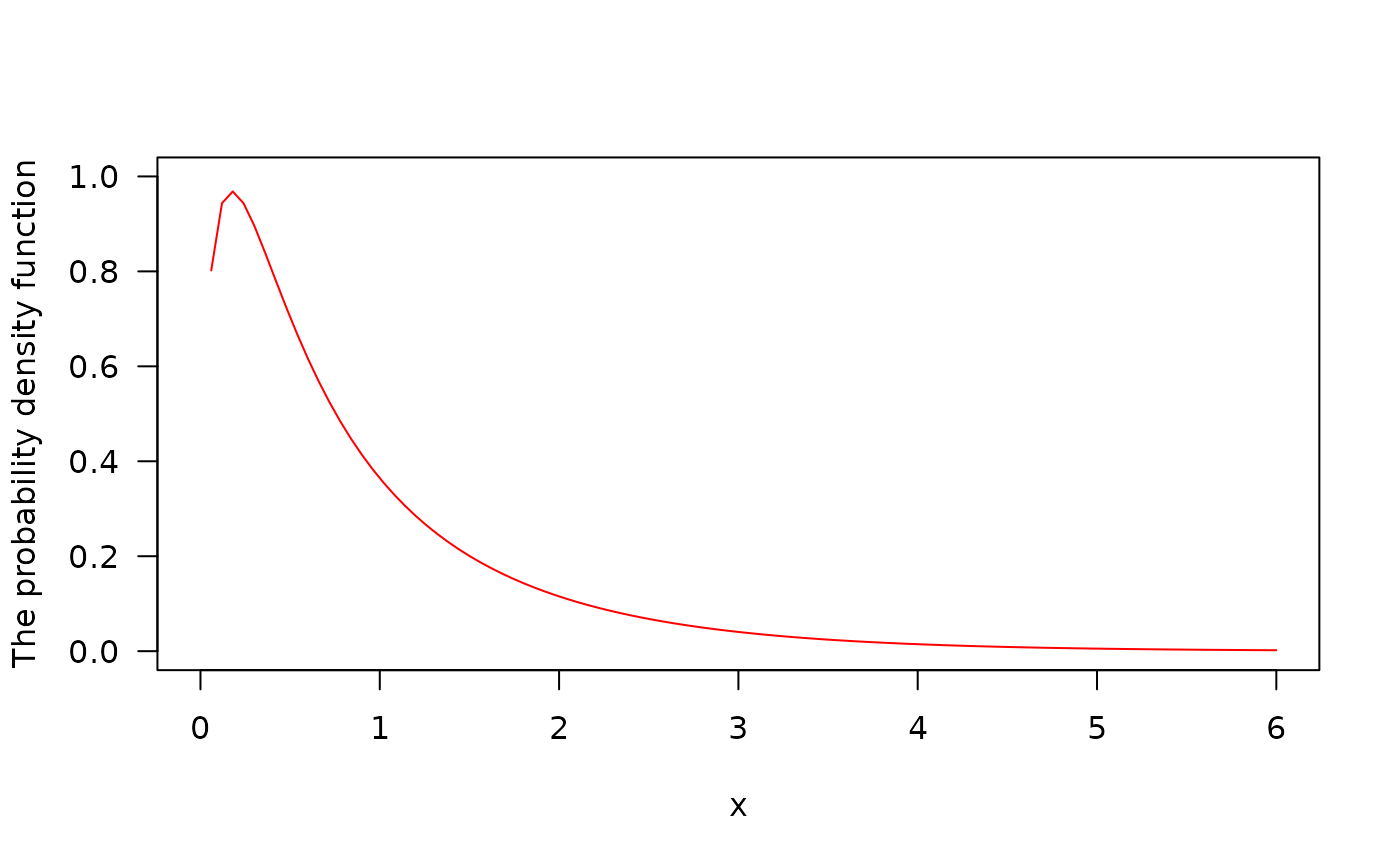
## The probability density function
curve(dWGEE(x, mu = 5, sigma = 0.5, nu = 1), from = 0, to = 6,
ylim = c(0, 1), col = "red", las = 1, ylab = "The probability density function")
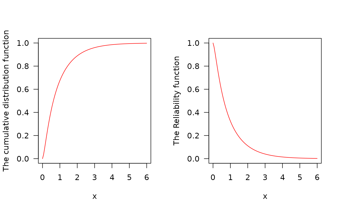
 ## The cumulative distribution and the Reliability function
par(mfrow = c(1, 2))
curve(pWGEE(x, mu = 5, sigma = 0.5, nu = 1), from = 0, to = 6,
ylim = c(0, 1), col = "red", las = 1, ylab = "The cumulative distribution function")
curve(pWGEE(x, mu = 5, sigma = 0.5, nu = 1, lower.tail = FALSE),
from = 0, to = 6, ylim = c(0, 1), col = "red", las = 1, ylab = "The Reliability function")
## The cumulative distribution and the Reliability function
par(mfrow = c(1, 2))
curve(pWGEE(x, mu = 5, sigma = 0.5, nu = 1), from = 0, to = 6,
ylim = c(0, 1), col = "red", las = 1, ylab = "The cumulative distribution function")
curve(pWGEE(x, mu = 5, sigma = 0.5, nu = 1, lower.tail = FALSE),
from = 0, to = 6, ylim = c(0, 1), col = "red", las = 1, ylab = "The Reliability function")
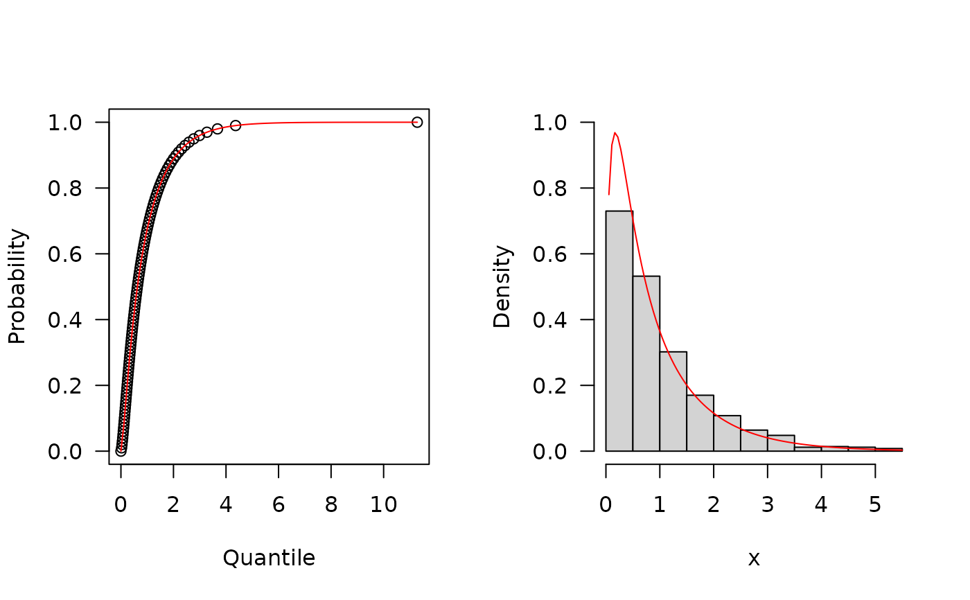
 ## The quantile function
p <- seq(from = 0, to = 0.99999, length.out = 100)
plot(x = qWGEE(p = p, mu = 5, sigma = 0.5, nu = 1), y = p,
xlab = "Quantile", las = 1, ylab = "Probability")
curve(pWGEE(x, mu = 5, sigma = 0.5, nu = 1), from = 0, add = TRUE,
col = "red")
## The random function
hist(rWGEE(1000, mu = 5, sigma = 0.5, nu = 1), freq = FALSE, xlab = "x",
ylim = c(0, 1), las = 1, main = "")
curve(dWGEE(x, mu = 5, sigma = 0.5, nu = 1), from = 0, add = TRUE,
col = "red", ylim = c(0, 1))
## The quantile function
p <- seq(from = 0, to = 0.99999, length.out = 100)
plot(x = qWGEE(p = p, mu = 5, sigma = 0.5, nu = 1), y = p,
xlab = "Quantile", las = 1, ylab = "Probability")
curve(pWGEE(x, mu = 5, sigma = 0.5, nu = 1), from = 0, add = TRUE,
col = "red")
## The random function
hist(rWGEE(1000, mu = 5, sigma = 0.5, nu = 1), freq = FALSE, xlab = "x",
ylim = c(0, 1), las = 1, main = "")
curve(dWGEE(x, mu = 5, sigma = 0.5, nu = 1), from = 0, add = TRUE,
col = "red", ylim = c(0, 1))
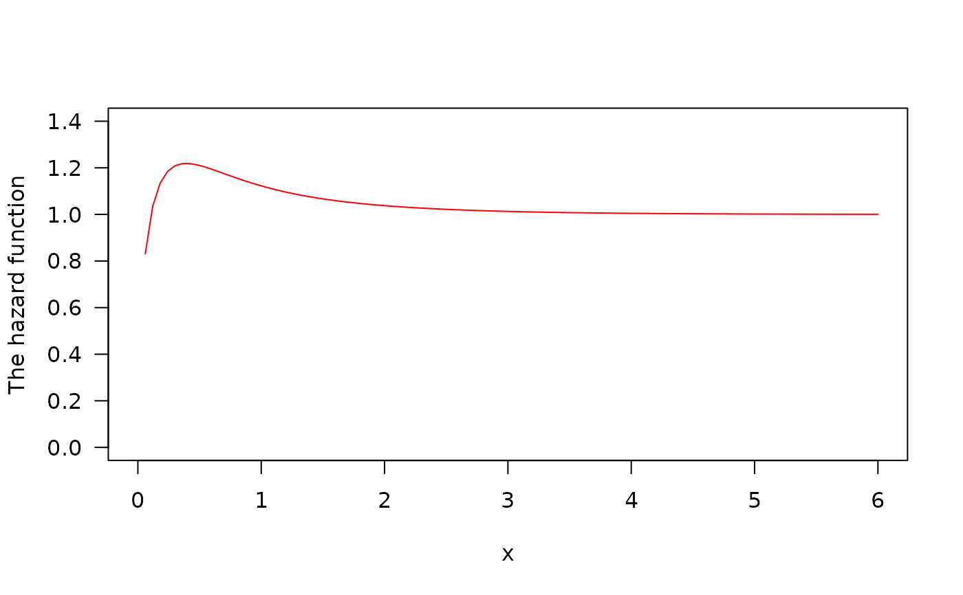
 ## The Hazard function(
par(mfrow=c(1,1))
curve(hWGEE(x, mu = 5, sigma = 0.5, nu = 1), from = 0, to = 6,
ylim = c(0, 1.4), col = "red", ylab = "The hazard function", las = 1)
## The Hazard function(
par(mfrow=c(1,1))
curve(hWGEE(x, mu = 5, sigma = 0.5, nu = 1), from = 0, to = 6,
ylim = c(0, 1.4), col = "red", ylab = "The hazard function", las = 1)
 par(old_par) # restore previous graphical parameters