Density, distribution function, quantile function,
random generation and hazard function for the weibull geometric distribution with
parameters mu, sigma and nu.
Usage
dWG(x, mu, sigma, nu, log = FALSE)

pWG(q, mu, sigma, nu, lower.tail = TRUE, log.p = FALSE)

qWG(p, sigma, mu, nu, lower.tail = TRUE, log.p = FALSE)

rWG(n, mu, sigma, nu)

hWG(x, mu, sigma, nu)
Arguments
- x, q
vector of quantiles.
- mu
scale parameter.
- sigma
shape parameter.
- nu
parameter of geometric random variable.
- log, log.p
logical; if TRUE, probabilities p are given as log(p).
- lower.tail
logical; if TRUE (default), probabilities are P[X <= x], otherwise, P[X > x].
- p
vector of probabilities.
- n
number of observations.
Value
dWG gives the density, pWG gives the distribution
function, qWG gives the quantile function, rWG
generates random deviates and hWG gives the hazard function.
Details
The Weibull geometric distribution with parameters mu,
sigma and nu has density given by
\(f(x) = (\sigma \mu^\sigma (1-\nu) x^(\sigma - 1) \exp(-(\mu x)^\sigma)) (1- \nu \exp(-(\mu x)^\sigma))^{-2},\)
for \(x > 0\), \(\mu > 0\), \(\sigma > 0\) and \(0 < \nu < 1\).
Author
Johan David Marin Benjumea, johand.marin@udea.edu.co
Examples
old_par <- par(mfrow = c(1, 1)) # save previous graphical parameters
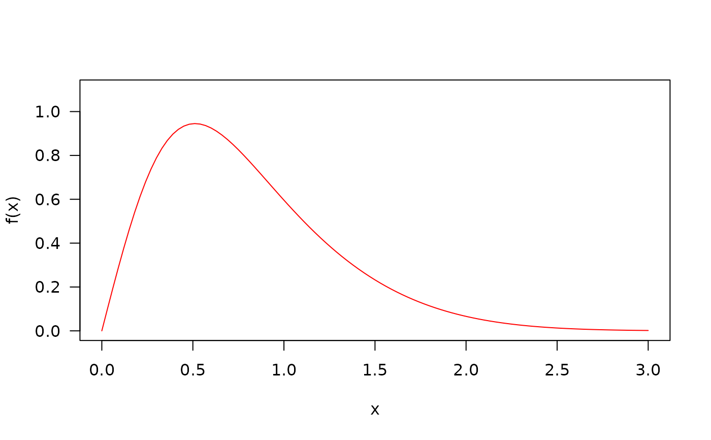
## The probability density function
curve(dWG(x, mu = 0.9, sigma = 2, nu = 0.5), from = 0, to = 3,
ylim = c(0, 1.1), col = "red", las = 1, ylab = "f(x)")
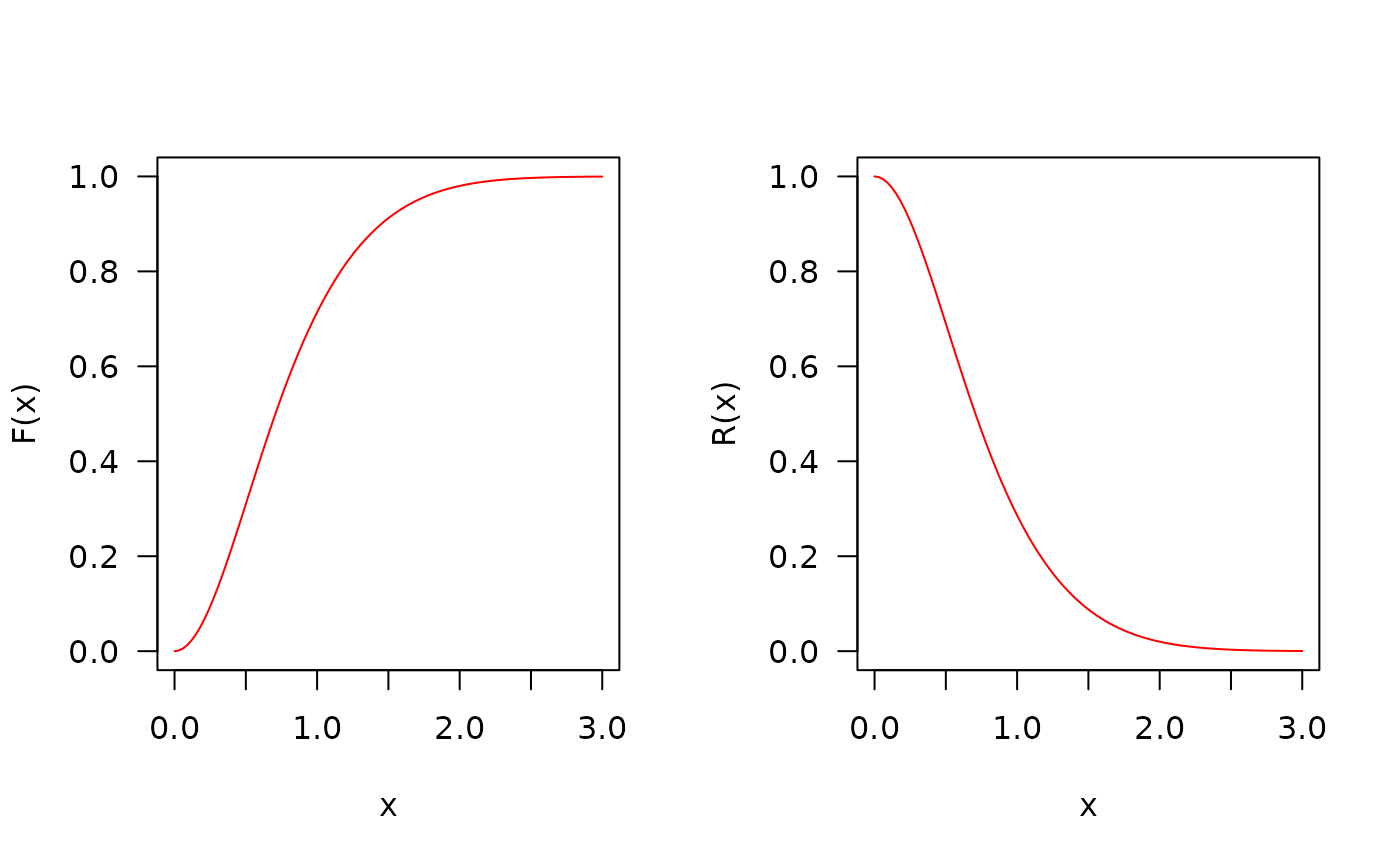
 ## The cumulative distribution and the Reliability function
par(mfrow = c(1, 2))
curve(pWG(x, mu = 0.9, sigma = 2, nu = 0.5), from = 0, to = 3,
ylim = c(0, 1), col = "red", las = 1, ylab = "F(x)")
curve(pWG(x, mu = 0.9, sigma = 2, nu = 0.5, lower.tail = FALSE),
from = 0, to = 3, ylim = c(0, 1), col = "red", las = 1, ylab = "R(x)")
## The cumulative distribution and the Reliability function
par(mfrow = c(1, 2))
curve(pWG(x, mu = 0.9, sigma = 2, nu = 0.5), from = 0, to = 3,
ylim = c(0, 1), col = "red", las = 1, ylab = "F(x)")
curve(pWG(x, mu = 0.9, sigma = 2, nu = 0.5, lower.tail = FALSE),
from = 0, to = 3, ylim = c(0, 1), col = "red", las = 1, ylab = "R(x)")
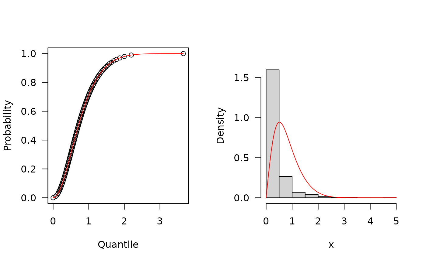
 ## The quantile function
p <- seq(from = 0, to = 0.99999, length.out = 100)
plot(x = qWG(p = p, mu = 0.9, sigma = 2, nu = 0.5), y = p,
xlab = "Quantile", las = 1, ylab = "Probability")
curve(pWG(x,mu = 0.9, sigma = 2, nu = 0.5), from = 0, add = TRUE,
col = "red")
## The random function
hist(rWG(1000, mu = 0.9, sigma = 2, nu = 0.5), freq = FALSE, xlab = "x",
ylim = c(0, 1.8), las = 1, main = "")
curve(dWG(x, mu = 0.9, sigma = 2, nu = 0.5), from = 0, add = TRUE,
col = "red", ylim = c(0, 1.8))
## The quantile function
p <- seq(from = 0, to = 0.99999, length.out = 100)
plot(x = qWG(p = p, mu = 0.9, sigma = 2, nu = 0.5), y = p,
xlab = "Quantile", las = 1, ylab = "Probability")
curve(pWG(x,mu = 0.9, sigma = 2, nu = 0.5), from = 0, add = TRUE,
col = "red")
## The random function
hist(rWG(1000, mu = 0.9, sigma = 2, nu = 0.5), freq = FALSE, xlab = "x",
ylim = c(0, 1.8), las = 1, main = "")
curve(dWG(x, mu = 0.9, sigma = 2, nu = 0.5), from = 0, add = TRUE,
col = "red", ylim = c(0, 1.8))
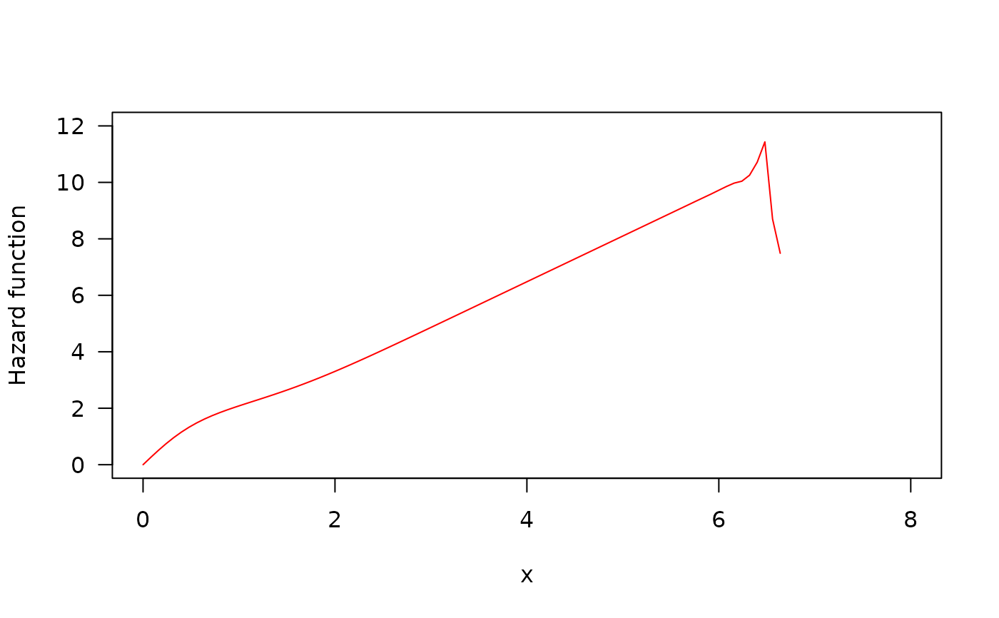
 ## The Hazard function(
par(mfrow=c(1,1))
curve(hWG(x, mu = 0.9, sigma = 2, nu = 0.5), from = 0, to = 8,
ylim = c(0, 12), col = "red", ylab = "Hazard function", las = 1)
## The Hazard function(
par(mfrow=c(1,1))
curve(hWG(x, mu = 0.9, sigma = 2, nu = 0.5), from = 0, to = 8,
ylim = c(0, 12), col = "red", ylab = "Hazard function", las = 1)
 par(old_par) # restore previous graphical parameters