Density, distribution function, quantile function,
random generation and hazard function for the Odd Weibull distribution with
parameters mu, sigma and nu.
Usage
dOW(x, mu, sigma, nu, log = FALSE)

pOW(q, mu, sigma, nu, lower.tail = TRUE, log.p = FALSE)

qOW(p, mu, sigma, nu, lower.tail = TRUE, log.p = FALSE)

rOW(n, mu, sigma, nu)

hOW(x, mu, sigma, nu)Value
dOW gives the density, pOW gives the distribution
function, qOW gives the quantile function, rOW
generates random deviates and hOW gives the hazard function.
Details
The Odd Weibull with parameters mu, sigma
and nu has density given by
\(f(x) = \left( \frac{\sigma\nu}{x} \right) (\mu x)^\sigma e^{(\mu x)^\sigma} \left(e^{(\mu x)^{\sigma}}-1\right)^{\nu-1} \left[ 1 + \left(e^{(\mu x)^{\sigma}}-1\right)^\nu \right]^{-2}\)
for x > 0.
Author
Jaime Mosquera Gutiérrez jmosquerag@unal.edu.co
Examples
old_par <- par(mfrow = c(1, 1)) # save previous graphical parameters
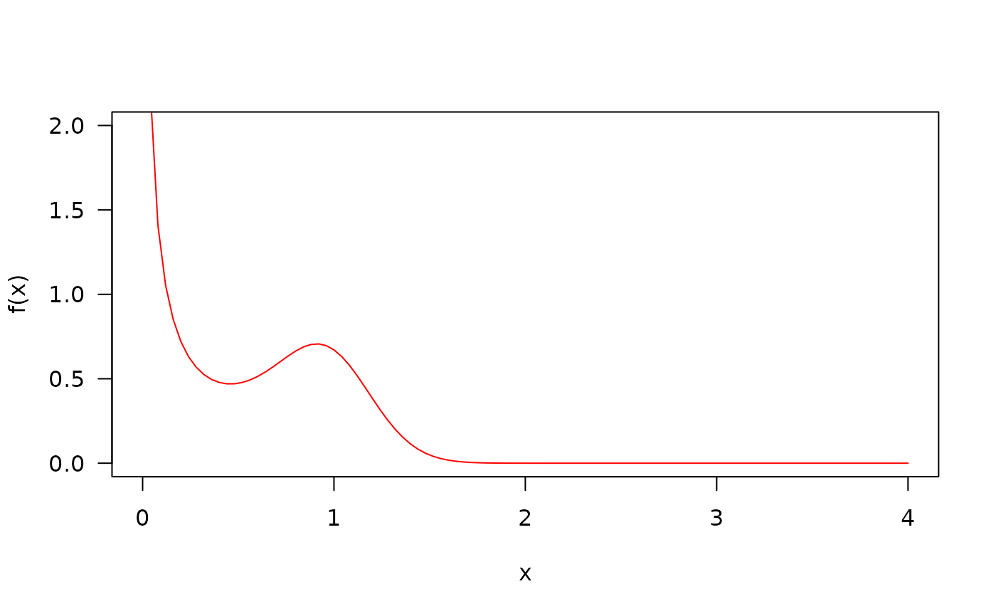
## The probability density function
curve(dOW(x, mu=2, sigma=3, nu=0.2), from=0, to=4, ylim=c(0, 2),
col="red", las=1, ylab="f(x)")
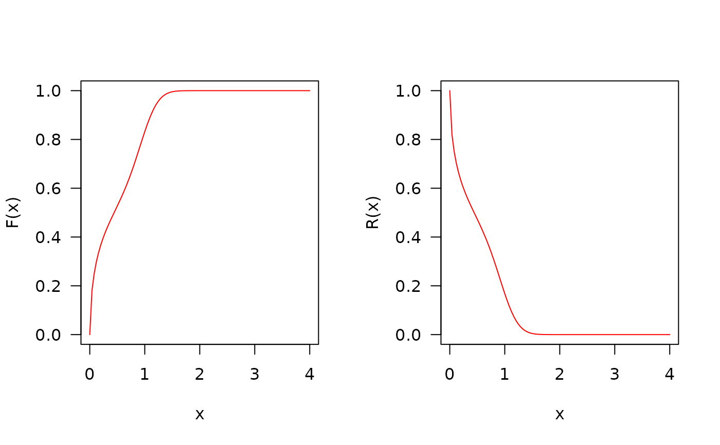
 ## The cumulative distribution and the Reliability function
par(mfrow = c(1, 2))
curve(pOW(x, mu=2, sigma=3, nu=0.2), from=0, to=4, ylim=c(0, 1),
col="red", las=1, ylab="F(x)")
curve(pOW(x, mu=2, sigma=3, nu=0.2, lower.tail=FALSE), from=0,
to=4, ylim=c(0, 1), col="red", las=1,
ylab = "R(x)")
## The cumulative distribution and the Reliability function
par(mfrow = c(1, 2))
curve(pOW(x, mu=2, sigma=3, nu=0.2), from=0, to=4, ylim=c(0, 1),
col="red", las=1, ylab="F(x)")
curve(pOW(x, mu=2, sigma=3, nu=0.2, lower.tail=FALSE), from=0,
to=4, ylim=c(0, 1), col="red", las=1,
ylab = "R(x)")
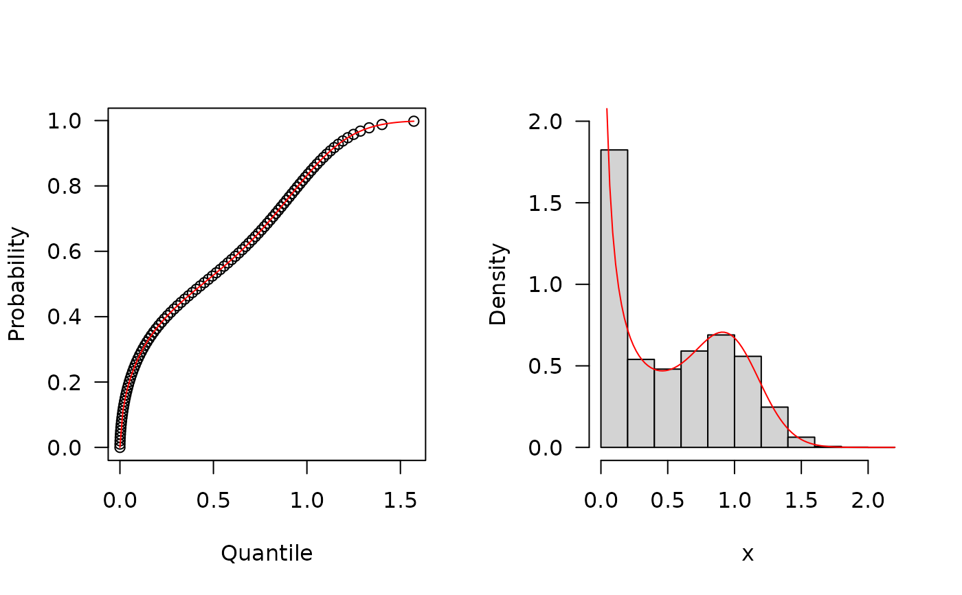
 ## The quantile function
p <- seq(from=0, to=0.998, length.out=100)
plot(x = qOW(p, mu=2, sigma=3, nu=0.2), y=p, xlab="Quantile", las=1,
ylab="Probability")
curve(pOW(x, mu=2, sigma=3, nu=0.2), from=0, add=TRUE, col="red")
## The random function
hist(rOW(n=10000, mu=2, sigma = 3, nu = 0.2), freq=FALSE, ylim = c(0, 2),
xlab = "x", las = 1, main = "")
curve(dOW(x, mu=2, sigma=3, nu=0.2), from=0, ylim=c(0, 2), add=TRUE,
col = "red")
## The quantile function
p <- seq(from=0, to=0.998, length.out=100)
plot(x = qOW(p, mu=2, sigma=3, nu=0.2), y=p, xlab="Quantile", las=1,
ylab="Probability")
curve(pOW(x, mu=2, sigma=3, nu=0.2), from=0, add=TRUE, col="red")
## The random function
hist(rOW(n=10000, mu=2, sigma = 3, nu = 0.2), freq=FALSE, ylim = c(0, 2),
xlab = "x", las = 1, main = "")
curve(dOW(x, mu=2, sigma=3, nu=0.2), from=0, ylim=c(0, 2), add=TRUE,
col = "red")
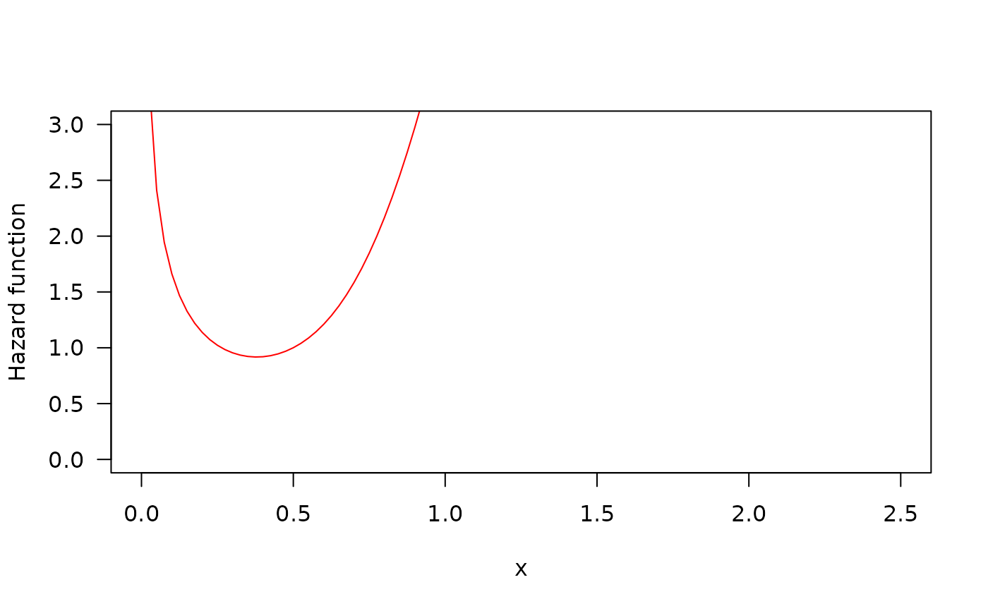
 ## The Hazard function
par(mfrow=c(1,1))
curve(hOW(x, mu=2, sigma=3, nu=0.2), from=0, to=2.5, ylim=c(0, 3),
col="red", ylab="Hazard function", las=1)
## The Hazard function
par(mfrow=c(1,1))
curve(hOW(x, mu=2, sigma=3, nu=0.2), from=0, to=2.5, ylim=c(0, 3),
col="red", ylab="Hazard function", las=1)
 par(old_par) # restore previous graphical parameters