Desnsity, distribution function, quantile function,
random generation and hazard function for the Marshall-Olkin Kappa distribution
with parameters mu, sigma, nu and tau.
Usage
dMOK(x, mu, sigma, nu, tau, log = FALSE)

pMOK(q, mu, sigma, nu, tau, lower.tail = TRUE, log.p = FALSE)

qMOK(p, mu, sigma, nu, tau, lower.tail = TRUE, log.p = FALSE)

rMOK(n, mu, sigma, nu, tau)

hMOK(x, mu, sigma, nu, tau)Value
dMOK gives the density, pMOK gives the distribution function,
qMOK gives the quantile function, rMOK generates random deviates
and hMOK gives the hazard function.
Details
The Marshall-Olkin Kappa distribution with parameters mu,
sigma, nu and tau has density given by:
\(f(x)=\frac{\tau\frac{\mu\nu}{\sigma}\left(\frac{x}{\sigma}\right)^{\nu-1} \left(\mu+\left(\frac{x}{\sigma}\right)^{\mu\nu}\right)^{-\frac{\mu+1}{\mu}}}{\left[\tau+(1-\tau)\left(\frac{\left(\frac{x}{\sigma}\right)^{\mu\nu}}{\mu+\left(\frac{x}{\sigma}\right)^{\mu\nu}}\right)^{\frac{1}{\mu}}\right]^2}\)
for x > 0.
Examples
old_par <- par(mfrow = c(1, 1)) # save previous graphical parameters
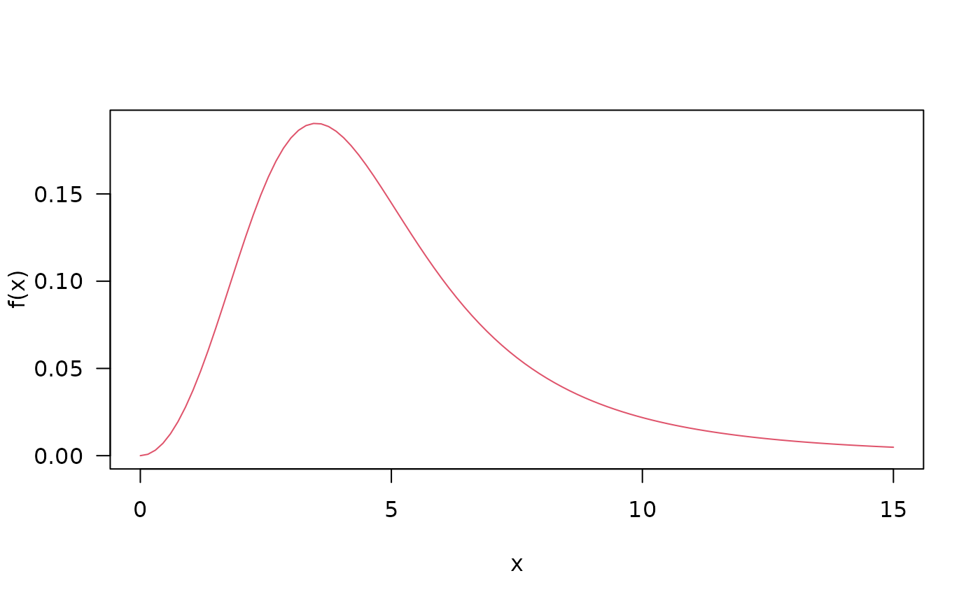
## The probability density function
par(mfrow = c(1,1))
curve(dMOK(x = x, mu = 1, sigma = 3.5, nu = 3, tau = 2), from = 0, to = 15,
ylab = 'f(x)', col = 2, las = 1)
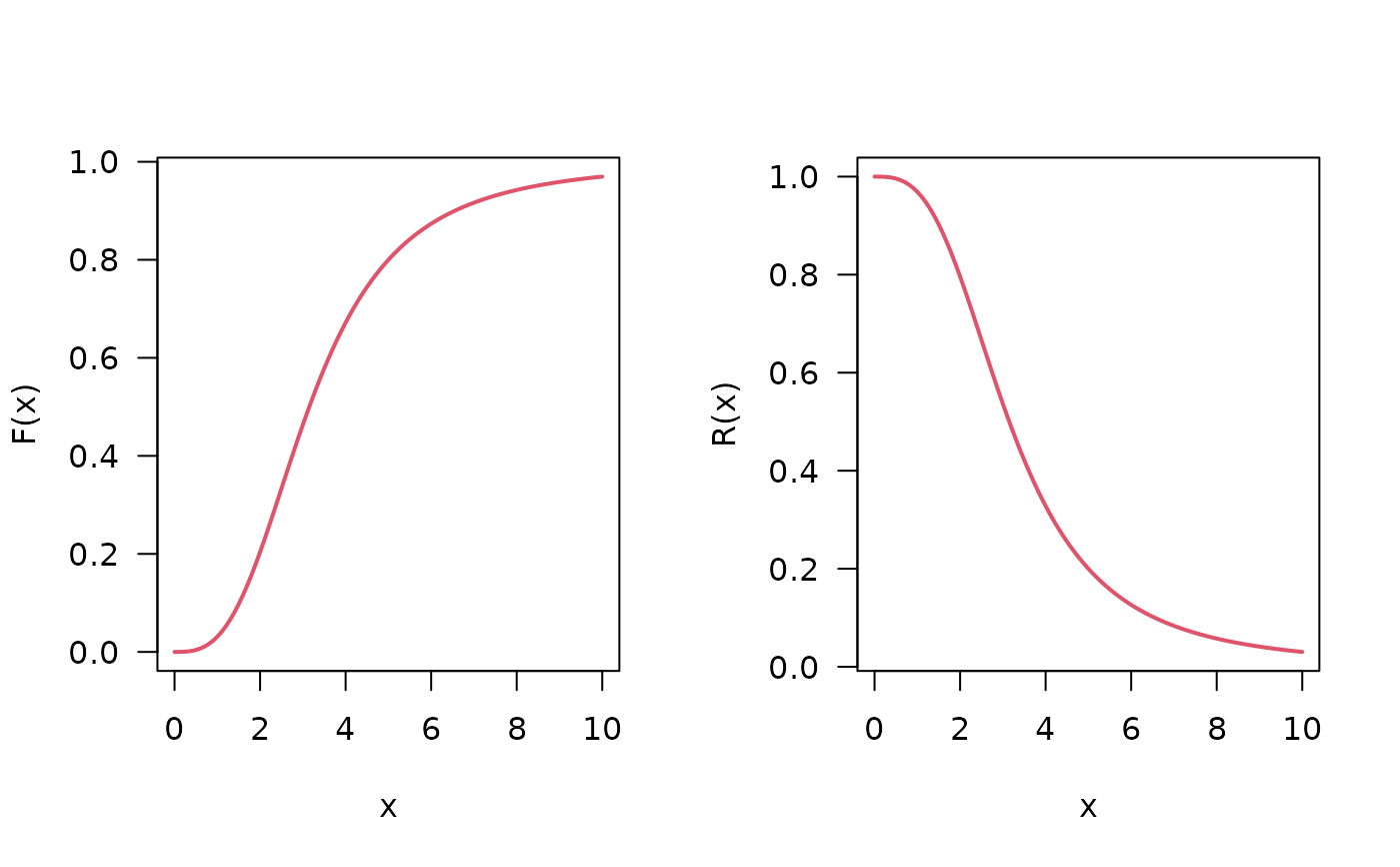
 ## The cumulative distribution and the Reliability function
par(mfrow = c(1,2))
curve(pMOK(q = x, mu = 1, sigma = 2.5, nu = 3, tau = 2), from = 0, to = 10,
col = 2, lwd = 2, las = 1, ylab = 'F(x)')
curve(pMOK(q = x, mu = 1, sigma = 2.5, nu = 3, tau = 2, lower.tail = FALSE), from = 0, to = 10,
col = 2, lwd = 2, las = 1, ylab = 'R(x)')
## The cumulative distribution and the Reliability function
par(mfrow = c(1,2))
curve(pMOK(q = x, mu = 1, sigma = 2.5, nu = 3, tau = 2), from = 0, to = 10,
col = 2, lwd = 2, las = 1, ylab = 'F(x)')
curve(pMOK(q = x, mu = 1, sigma = 2.5, nu = 3, tau = 2, lower.tail = FALSE), from = 0, to = 10,
col = 2, lwd = 2, las = 1, ylab = 'R(x)')
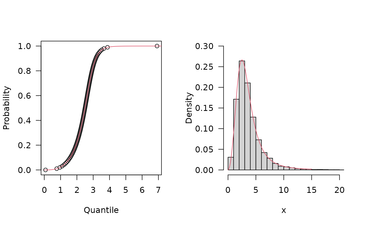
 ## The quantile function
p <- seq(from = 0.00001, to = 0.99999, length.out = 100)
plot(x = qMOK(p = p, mu = 4, sigma = 2.5, nu = 3, tau = 2), y = p, xlab = 'Quantile',
las = 1, ylab = 'Probability')
curve(pMOK(q = x, mu = 4, sigma = 2.5, nu = 3, tau = 2), from = 0, to = 15,
add = TRUE, col = 2)
## The random function
hist(rMOK(n = 10000, mu = 1, sigma = 2.5, nu = 3, tau = 2), freq = FALSE,
xlab = "x", las = 1, main = '', ylim = c(0,.3), xlim = c(0,20), breaks = 50)
curve(dMOK(x, mu = 1, sigma = 2.5, nu = 3, tau = 2), from = 0, to = 15, add = TRUE, col = 2)
## The quantile function
p <- seq(from = 0.00001, to = 0.99999, length.out = 100)
plot(x = qMOK(p = p, mu = 4, sigma = 2.5, nu = 3, tau = 2), y = p, xlab = 'Quantile',
las = 1, ylab = 'Probability')
curve(pMOK(q = x, mu = 4, sigma = 2.5, nu = 3, tau = 2), from = 0, to = 15,
add = TRUE, col = 2)
## The random function
hist(rMOK(n = 10000, mu = 1, sigma = 2.5, nu = 3, tau = 2), freq = FALSE,
xlab = "x", las = 1, main = '', ylim = c(0,.3), xlim = c(0,20), breaks = 50)
curve(dMOK(x, mu = 1, sigma = 2.5, nu = 3, tau = 2), from = 0, to = 15, add = TRUE, col = 2)
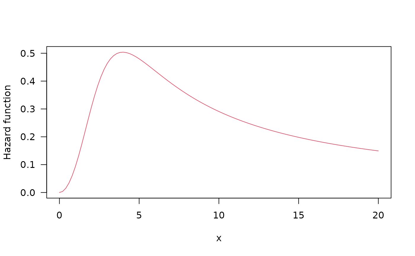
 ## The Hazard function
par(mfrow = c(1,1))
curve(hMOK(x = x, mu = 1, sigma = 2.5, nu = 3, tau = 2), from = 0, to = 20,
col = 2, ylab = 'Hazard function', las = 1)
## The Hazard function
par(mfrow = c(1,1))
curve(hMOK(x = x, mu = 1, sigma = 2.5, nu = 3, tau = 2), from = 0, to = 20,
col = 2, ylab = 'Hazard function', las = 1)
 par(old_par) # restore previous graphical parameters