Density, distribution function, quantile function,
random generation and hazard function for the Marshall-Olkin Extended Inverse Weibull distribution
with parameters mu, sigma and nu.
Usage
dMOEIW(x, mu, sigma, nu, log = FALSE)

pMOEIW(q, mu, sigma, nu, lower.tail = TRUE, log.p = FALSE)

qMOEIW(p, mu, sigma, nu, lower.tail = TRUE, log.p = FALSE)

rMOEIW(n, mu, sigma, nu)

hMOEIW(x, mu, sigma, nu)Value
dMOEIW gives the density, pMOEIW gives the distribution
function, qMOEIW gives the quantile function, rMOEIW
generates random deviates and hMOEIW gives the hazard function.
Details
The Marshall-Olkin Extended Inverse Weibull distribution mu,
sigma and nu has density given by
\(f(x) = \frac{\mu \sigma \nu x^{-(\sigma + 1)} exp\{{-\mu x^{-\sigma}}\}}{\{\nu -(\nu-1) exp\{{-\mu x ^{-\sigma}}\} \}^{2}},\)
for x > 0.
Author
Amylkar Urrea Montoya, amylkar.urrea@udea.edu.co
Examples
old_par <- par(mfrow = c(1, 1)) # save previous graphical parameters
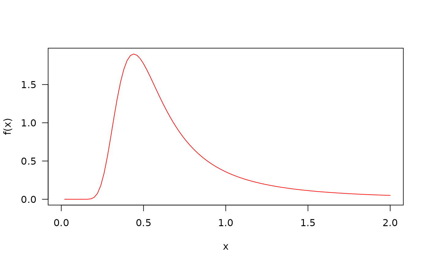
## The probability density function
curve(dMOEIW(x, mu=0.6, sigma=1.7, nu=0.3), from=0, to=2,
col="red", ylab="f(x)", las=1)
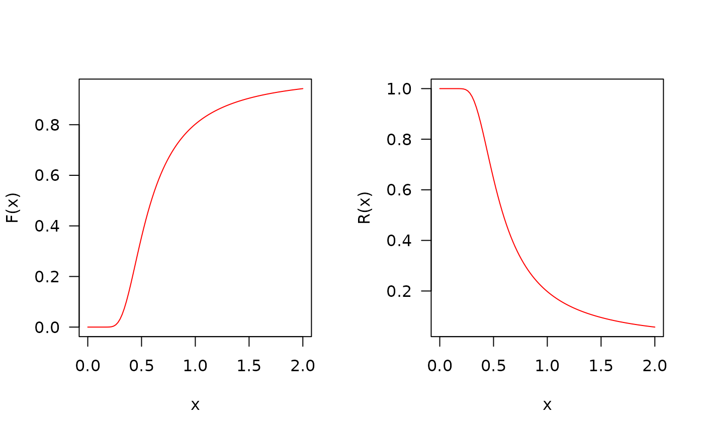
 ## The cumulative distribution and the Reliability function
par(mfrow=c(1, 2))
curve(pMOEIW(x, mu=0.6, sigma=1.7, nu=0.3),
from=0.0001, to=2, col="red", las=1, ylab="F(x)")
curve(pMOEIW(x, mu=0.6, sigma=1.7, nu=0.3, lower.tail=FALSE),
from=0.0001, to=2, col="red", las=1, ylab="R(x)")
## The cumulative distribution and the Reliability function
par(mfrow=c(1, 2))
curve(pMOEIW(x, mu=0.6, sigma=1.7, nu=0.3),
from=0.0001, to=2, col="red", las=1, ylab="F(x)")
curve(pMOEIW(x, mu=0.6, sigma=1.7, nu=0.3, lower.tail=FALSE),
from=0.0001, to=2, col="red", las=1, ylab="R(x)")
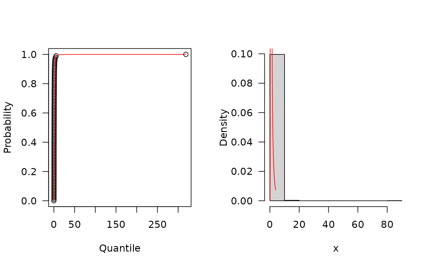
 ## The quantile function
p <- seq(from=0, to=0.99999, length.out=100)
plot(x=qMOEIW(p, mu=0.6, sigma=1.7, nu=0.3), y=p, xlab="Quantile",
las=1, ylab="Probability")
curve(pMOEIW(x, mu=0.6, sigma=1.7, nu=0.3),
from=0, add=TRUE, col="red")
## The random function
hist(rMOEIW(n=1000, mu=0.6, sigma=1.7, nu=0.3), freq=FALSE,
xlab="x", las=1, main="")
curve(dMOEIW(x, mu=0.6, sigma=1.7, nu=0.3),
from=0.001, to=4, add=TRUE, col="red")
## The quantile function
p <- seq(from=0, to=0.99999, length.out=100)
plot(x=qMOEIW(p, mu=0.6, sigma=1.7, nu=0.3), y=p, xlab="Quantile",
las=1, ylab="Probability")
curve(pMOEIW(x, mu=0.6, sigma=1.7, nu=0.3),
from=0, add=TRUE, col="red")
## The random function
hist(rMOEIW(n=1000, mu=0.6, sigma=1.7, nu=0.3), freq=FALSE,
xlab="x", las=1, main="")
curve(dMOEIW(x, mu=0.6, sigma=1.7, nu=0.3),
from=0.001, to=4, add=TRUE, col="red")
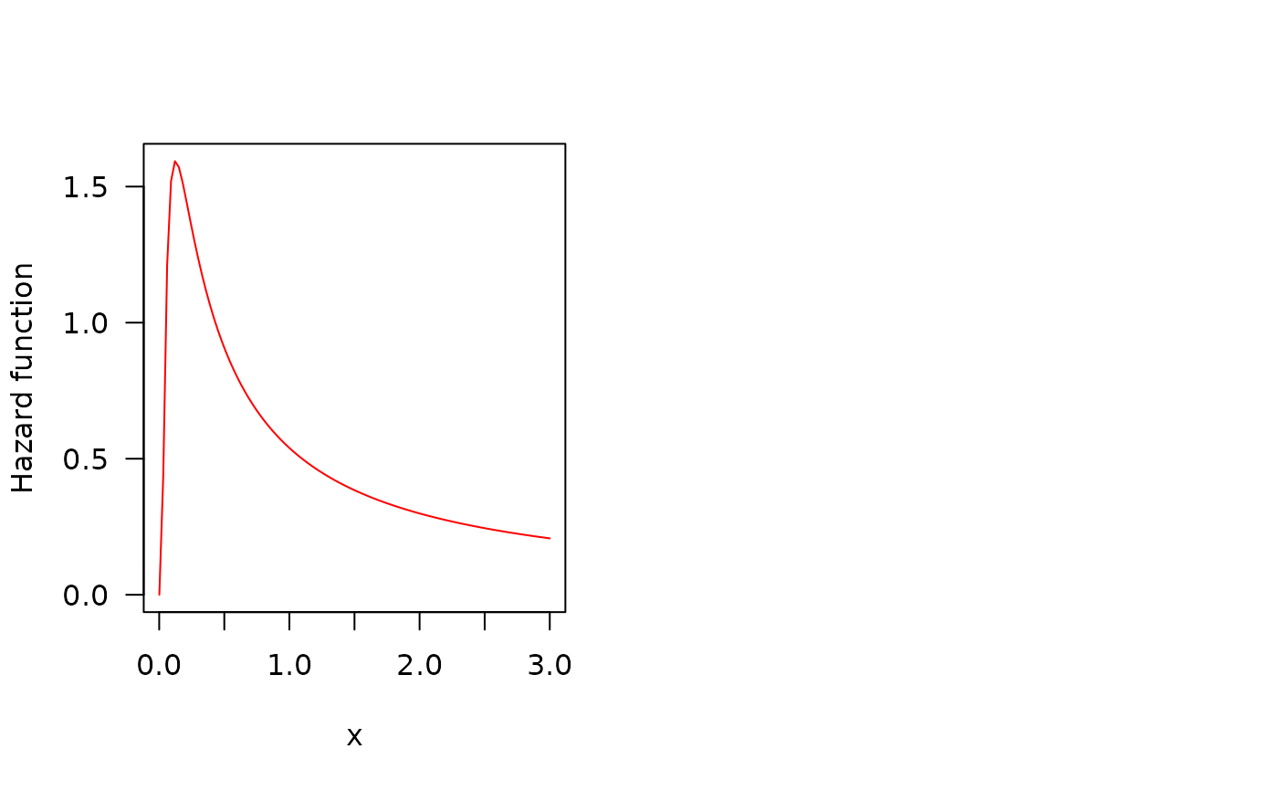
 ## The Hazard function
curve(hMOEIW(x, mu=0.5, sigma=0.7, nu=1), from=0.001, to=3,
col="red", ylab="Hazard function", las=1)
par(old_par) # restore previous graphical parameters
## The Hazard function
curve(hMOEIW(x, mu=0.5, sigma=0.7, nu=1), from=0.001, to=3,
col="red", ylab="Hazard function", las=1)
par(old_par) # restore previous graphical parameters