The Log-Weibull distribution

Density, distribution function, quantile function, random generation and hazard function for the Log-Weibull distribution with parameters mu and sigma.

Usage

dLW(x, mu, sigma, log = FALSE)

pLW(q, mu, sigma, lower.tail = TRUE, log.p = FALSE)

qLW(p, mu, sigma, lower.tail = TRUE, log.p = FALSE)

rLW(n, mu, sigma)

hLW(x, mu, sigma)

Arguments

x, q

vector of quantiles.

mu

parameter.

sigma

parameter.

log, log.p

logical; if TRUE, probabilities p are given as log(p).

lower.tail

logical; if TRUE (default), probabilities are P[X <= x], otherwise, P[X > x].

p

vector of probabilities.

n

number of observations.

Value

dLW gives the density, pLW gives the distribution function, qLW gives the quantile function, rLW generates random deviates and hLW gives the hazard function.

Details

The Log-Weibull Distribution with parameters mu and sigma has density given by

\(f(y)=(1/\sigma) e^{((y - \mu)/\sigma)} exp\{-e^{((y - \mu)/\sigma)}\},\)

for - infty < y < infty.

References

Almalki SJ, Nadarajah S (2014). “Modifications of the Weibull distribution: A review.” Reliability Engineering & System Safety, 124, 32–55. doi:10.1016/j.ress.2013.11.010 .

E.J G (1958). Statistics of extremes. Columbia University Press. ISBN 10:0231021909.

Author

Amylkar Urrea Montoya, amylkar.urrea@udea.edu.co

Examples

old_par <- par(mfrow = c(1, 1)) # save previous graphical parameters

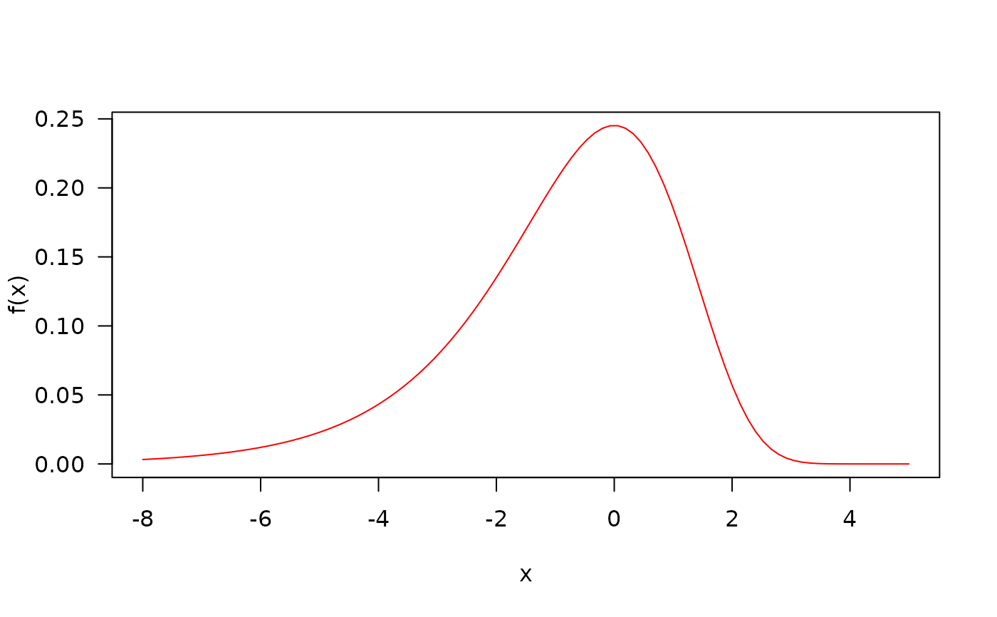
## The probability density function
curve(dLW(x, mu=0, sigma=1.5), from=-8, to=5,
      col="red", las=1, ylab="f(x)")


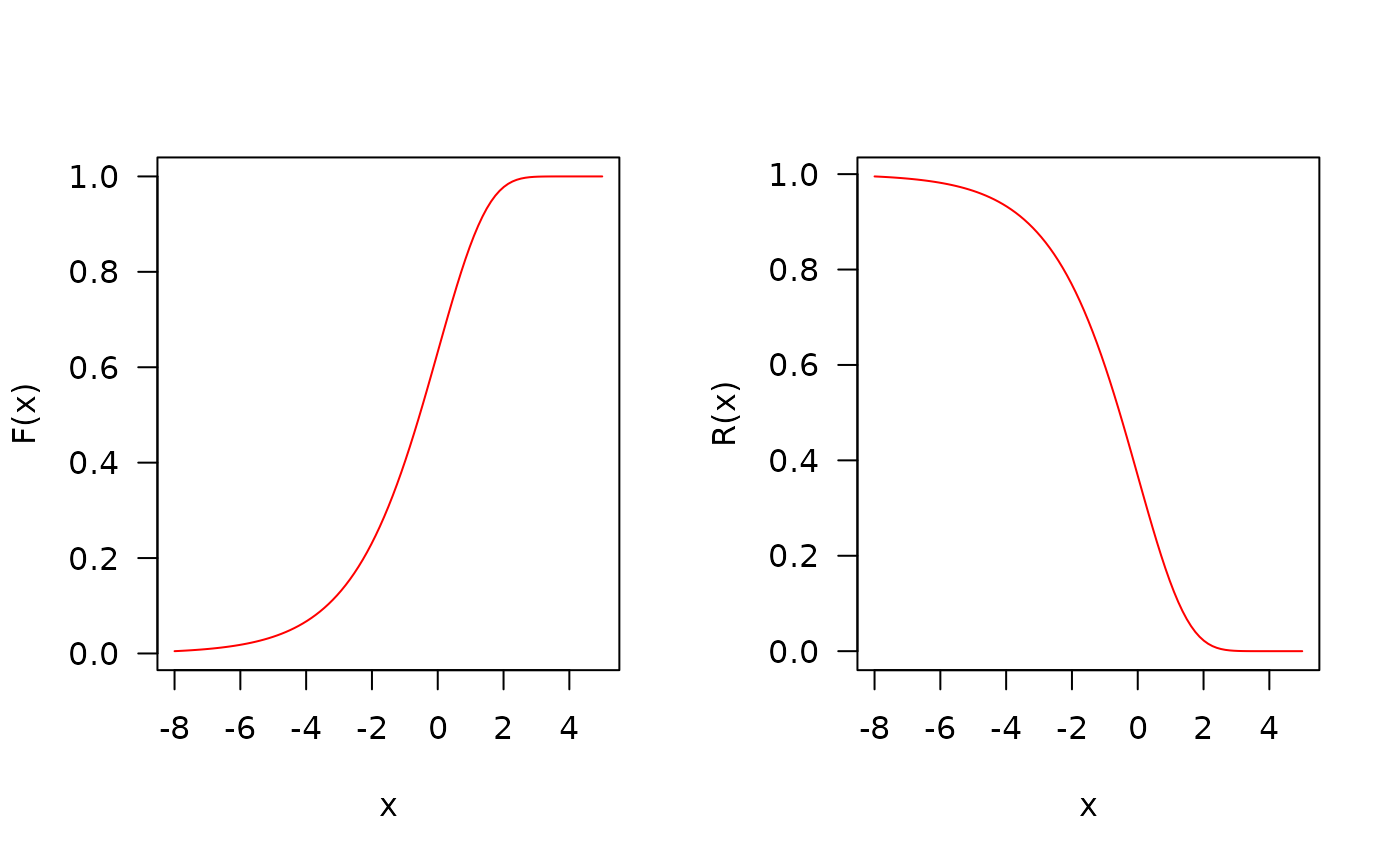
## The cumulative distribution and the Reliability function
par(mfrow=c(1, 2))
curve(pLW(x, mu=0, sigma=1.5),
      from=-8, to=5,  col="red", las=1, ylab="F(x)")
curve(pLW(x, mu=0, sigma=1.5, lower.tail=FALSE),
      from=-8, to=5, col="red", las=1, ylab="R(x)")


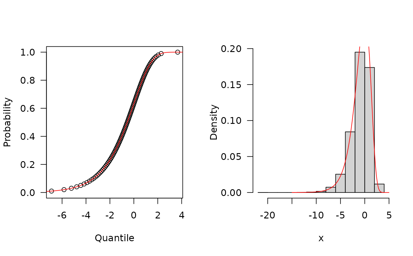
## The quantile function
p <- seq(from=0, to=0.99999, length.out=100)
plot(x=qLW(p, mu=0, sigma=1.5), y=p, xlab="Quantile",
     las=1, ylab="Probability")
curve(pLW(x, mu=0, sigma=1.5), from=-8, to=5, add=TRUE, col="red")

## The random function
hist(rLW(n=10000, mu=0, sigma=1.5), freq=FALSE,
     xlab="x", las=1, main="")
curve(dLW(x, mu=0, sigma=1.5), from=-15, to=6, add=TRUE, col="red")


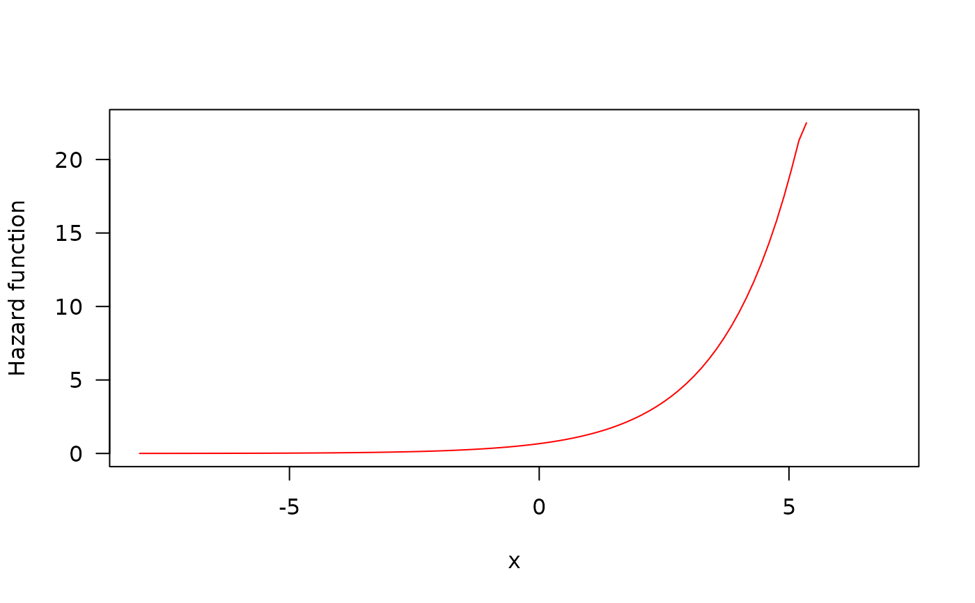
## The Hazard function
par(mfrow=c(1,1))
curve(hLW(x, mu=0, sigma=1.5), from=-8, to=7,
      col="red", ylab="Hazard function", las=1)


par(old_par) # restore previous graphical parameters