Density, distribution function, quantile function,
random generation and hazard function for the Kumaraswamy Inverse Weibull distribution
with parameters mu, sigma and nu.
Usage
dKumIW(x, mu, sigma, nu, log = FALSE)

pKumIW(q, mu, sigma, nu, lower.tail = TRUE, log.p = FALSE)

qKumIW(p, mu, sigma, nu, lower.tail = TRUE, log.p = FALSE)

rKumIW(n, mu, sigma, nu)

hKumIW(x, mu, sigma, nu)Value
dKumIW gives the density, pKumIW gives the distribution
function, qKumIW gives the quantile function, rKumIW
generates random deviates and hKumIW gives the hazard function.
Details
The Kumaraswamy Inverse Weibull Distribution with parameters mu,
sigma and nu has density given by
\(f(x)= \mu \sigma \nu x^{-\sigma - 1} \exp{- \mu x^{-\sigma}} (1 - \exp{- \mu x^{-\sigma}})^{\nu - 1},\)
for \(x > 0\), \(\mu > 0\), \(\sigma > 0\) and \(\nu > 0\).
The KumIW distribution with \(\nu=1\) corresponds with the IW distribution.
Author
Freddy Hernandez, fhernanb@unal.edu.co
Examples
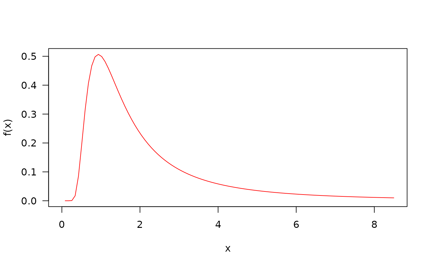
# The probability density function
curve(dKumIW(x, mu=1.5, sigma=2.3, nu=1.7), from=0, to=8,
col="red", las=1, ylab="f(x)")
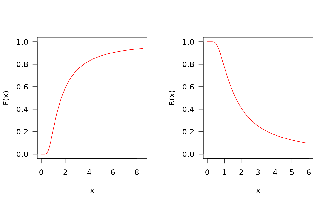
 # The cumulative distribution and the Reliability function
par(mfrow=c(1, 2))
curve(pKumIW(x, mu=1.5, sigma=2.3, nu=1.7), from=0, to=8,
ylim=c(0, 1), col="red", las=1, ylab="F(x)")
curve(pKumIW(x, mu=1.5, sigma=2.3, nu=1.7, lower.tail=FALSE),
from=0, to=8, ylim=c(0, 1), col="red", las=1, ylab="R(x)")
# The cumulative distribution and the Reliability function
par(mfrow=c(1, 2))
curve(pKumIW(x, mu=1.5, sigma=2.3, nu=1.7), from=0, to=8,
ylim=c(0, 1), col="red", las=1, ylab="F(x)")
curve(pKumIW(x, mu=1.5, sigma=2.3, nu=1.7, lower.tail=FALSE),
from=0, to=8, ylim=c(0, 1), col="red", las=1, ylab="R(x)")
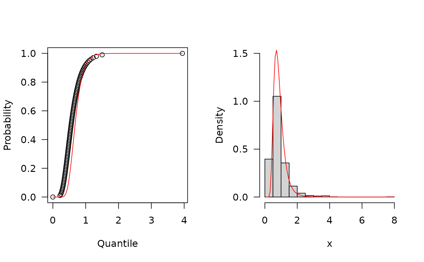
 # The quantile function
p <- seq(from=0, to=0.99, length.out=100)
plot(x=qKumIW(p=p, mu=1.5, sigma=2.3, nu=1.7), y=p,
xlab="Quantile", las=1, ylab="Probability")
curve(pKumIW(x, mu=1.5, sigma=2.3, nu=1.7),
from=0, add=TRUE, col="red")
# The random function
hist(rKumIW(1000, mu=1.5, sigma=2.3, nu=1.7), freq=FALSE,
xlab="x", las=1, main="", xlim=c(0, 8))
curve(dKumIW(x, mu=1.5, sigma=2.3, nu=1.7), from=0, to=8, add=TRUE,
col="red")
# The quantile function
p <- seq(from=0, to=0.99, length.out=100)
plot(x=qKumIW(p=p, mu=1.5, sigma=2.3, nu=1.7), y=p,
xlab="Quantile", las=1, ylab="Probability")
curve(pKumIW(x, mu=1.5, sigma=2.3, nu=1.7),
from=0, add=TRUE, col="red")
# The random function
hist(rKumIW(1000, mu=1.5, sigma=2.3, nu=1.7), freq=FALSE,
xlab="x", las=1, main="", xlim=c(0, 8))
curve(dKumIW(x, mu=1.5, sigma=2.3, nu=1.7), from=0, to=8, add=TRUE,
col="red")
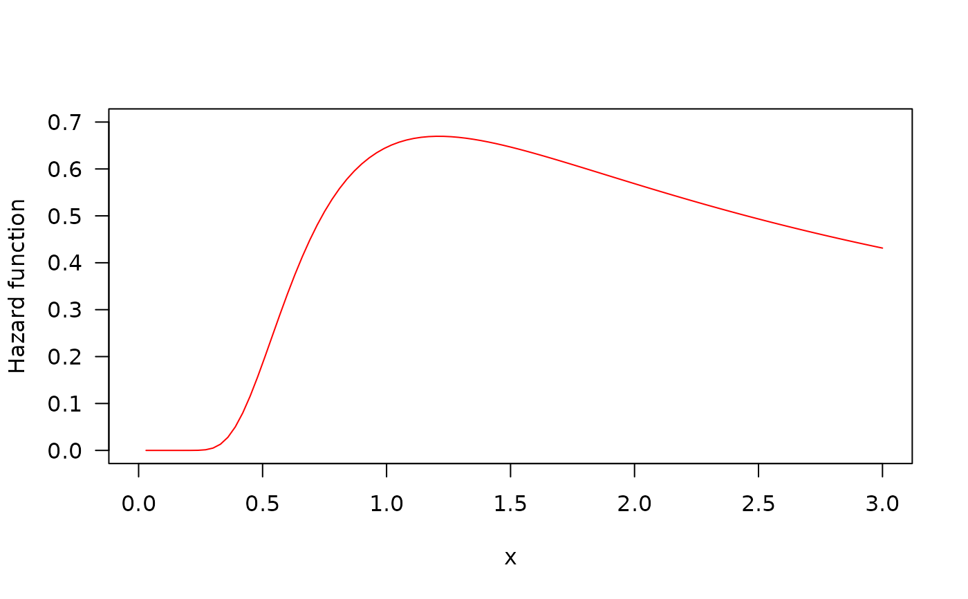
 # The Hazard function
par(mfrow=c(1, 1))
curve(hKumIW(x, mu=1.5, sigma=2.3, nu=1.7), from=0, to=8,
col="red", ylab="Hazard function", las=1)
# The Hazard function
par(mfrow=c(1, 1))
curve(hKumIW(x, mu=1.5, sigma=2.3, nu=1.7), from=0, to=8,
col="red", ylab="Hazard function", las=1)