The Inverse Weibull distribution

Density, distribution function, quantile function, random generation and hazard function for the inverse weibull distribution with parameters mu and sigma.

Usage

dIW(x, mu, sigma, log = FALSE)

pIW(q, mu, sigma, lower.tail = TRUE, log.p = FALSE)

qIW(p, mu, sigma, lower.tail = TRUE, log.p = FALSE)

rIW(n, mu, sigma)

hIW(x, mu, sigma)

Arguments

x, q

vector of quantiles.

mu

scale parameter.

sigma

shape parameters.

log, log.p

logical; if TRUE, probabilities p are given as log(p).

lower.tail

logical; if TRUE (default), probabilities are P[X <= x], otherwise, P[X > x].

p

vector of probabilities.

n

number of observations.

Value

dIW gives the density, pIW gives the distribution function, qIW gives the quantile function, rIW generates random deviates and hIW gives the hazard function.

Details

The inverse weibull distribution with parameters mu and sigma has density given by

\(f(x) = \mu \sigma x^{-\sigma-1} \exp(-\mu x^{-\sigma})\)

for \(x > 0\), \(\mu > 0\) and \(\sigma > 0\)

References

almalki2014modificationsRelDists

drapella1993complementaryRelDists

Author

Freddy Hernandez, fhernanb@unal.edu.co

Examples

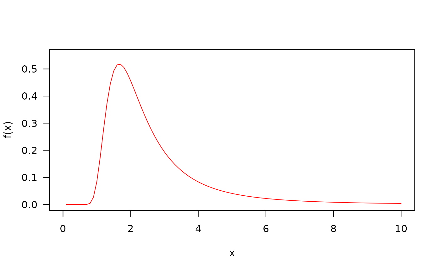
# The probability density function
curve(dIW(x, mu=1, sigma=2), from=0, to=10,
      col="red", las=1, ylab="f(x)")


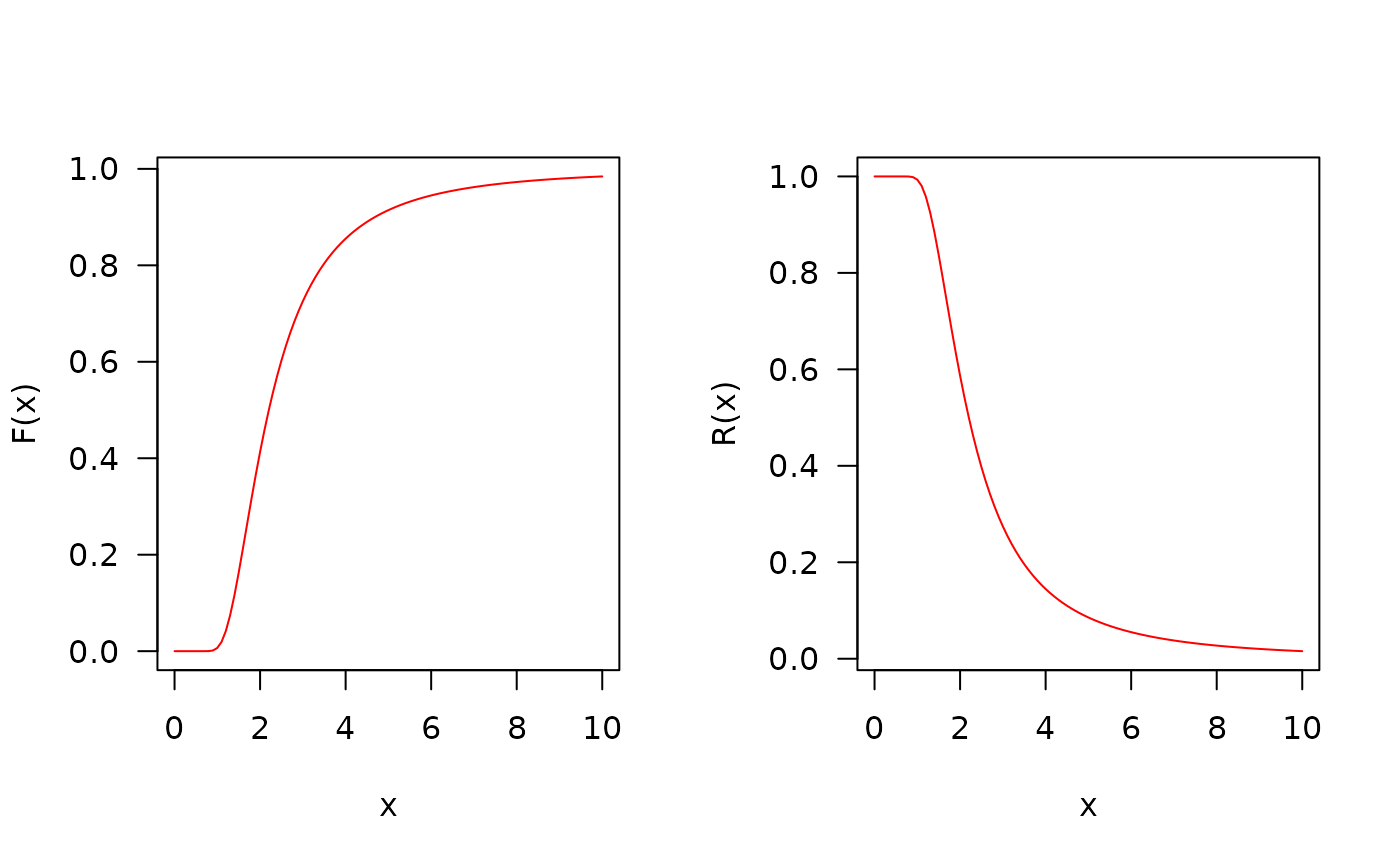
# The cumulative distribution and the Reliability function
par(mfrow=c(1, 2))
curve(pIW(x, mu=1, sigma=2),
      from=0, to=10,  col="red", las=1, ylab="F(x)")
curve(pIW(x, mu=1, sigma=2, lower.tail=FALSE),
      from=0, to=10, col="red", las=1, ylab="R(x)")

            
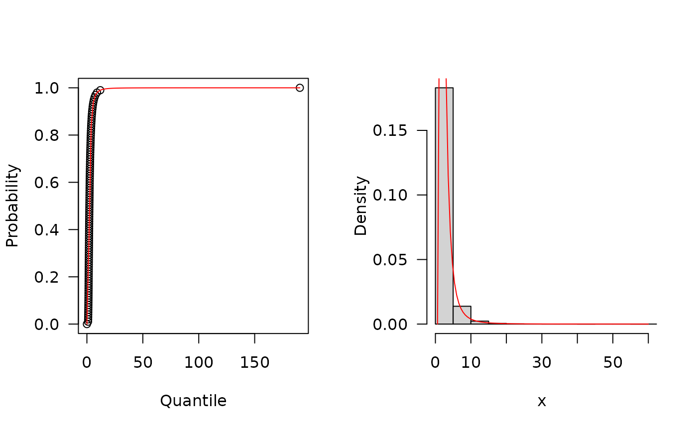
# The quantile function
p <- seq(from=0, to=0.99, length.out=100)
plot(x=qIW(p, mu=1, sigma=2), y=p, xlab="Quantile",
  las=1, ylab="Probability")
curve(pIW(x, mu=1, sigma=2), from=0, add=TRUE, col="red")
  
# The random function
hist(rIW(n=1000, mu=1, sigma=2), freq=FALSE, xlim=c(0, 40),
  xlab="x", las=1, main="")
curve(dIW(x, mu=1, sigma=2), from=0, add=TRUE, col="red")


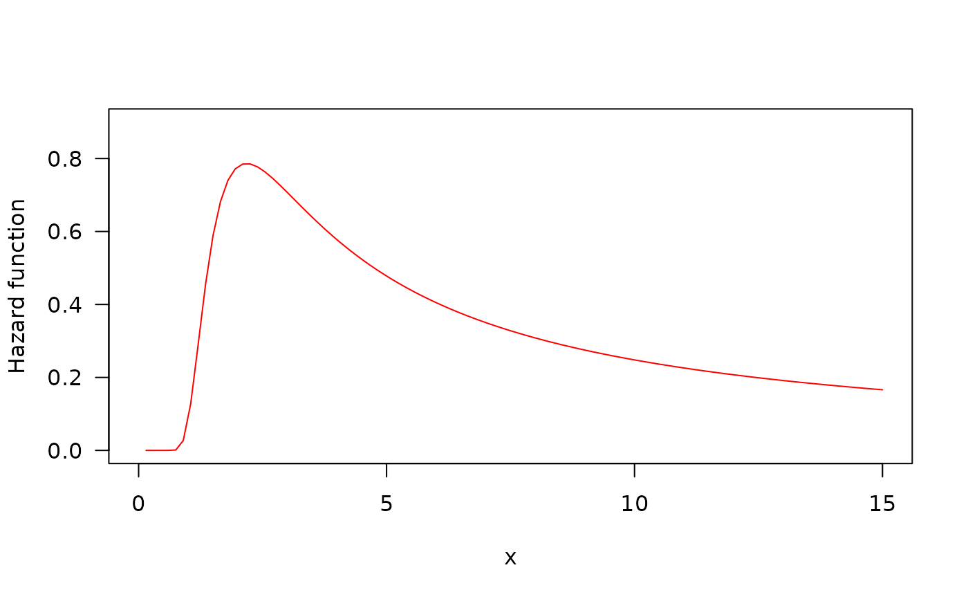
# The Hazard function
par(mfrow=c(1, 1))
curve(hIW(x, mu=1, sigma=2), from=0, to=15,
   col="red", ylab="Hazard function", las=1)