Density, distribution function, quantile function,
random generation and hazard function for the Generalized Inverse Weibull distribution
with parameters mu, sigma and nu.
Usage
dGIW(x, mu, sigma, nu, log = FALSE)

pGIW(q, mu, sigma, nu, lower.tail = TRUE, log.p = FALSE)

qGIW(p, mu, sigma, nu, lower.tail = TRUE, log.p = FALSE)

rGIW(n, mu, sigma, nu)

hGIW(x, mu, sigma, nu)Value
dGIW gives the density, pGIW gives the distribution
function, qGIW gives the quantile function, rGIW
generates random deviates and hGIW gives the hazard function.
Details
The Generalized Inverse Weibull distribution mu,
sigma and nu has density given by
\(f(x) = \nu \sigma \mu^{\sigma} x^{-(\sigma + 1)} exp \{-\nu (\frac{\mu}{x})^{\sigma}\},\)
for x > 0.
Author
Amylkar Urrea Montoya, amylkar.urrea@udea.edu.co
Examples
old_par <- par(mfrow = c(1, 1)) # save previous graphical parameters
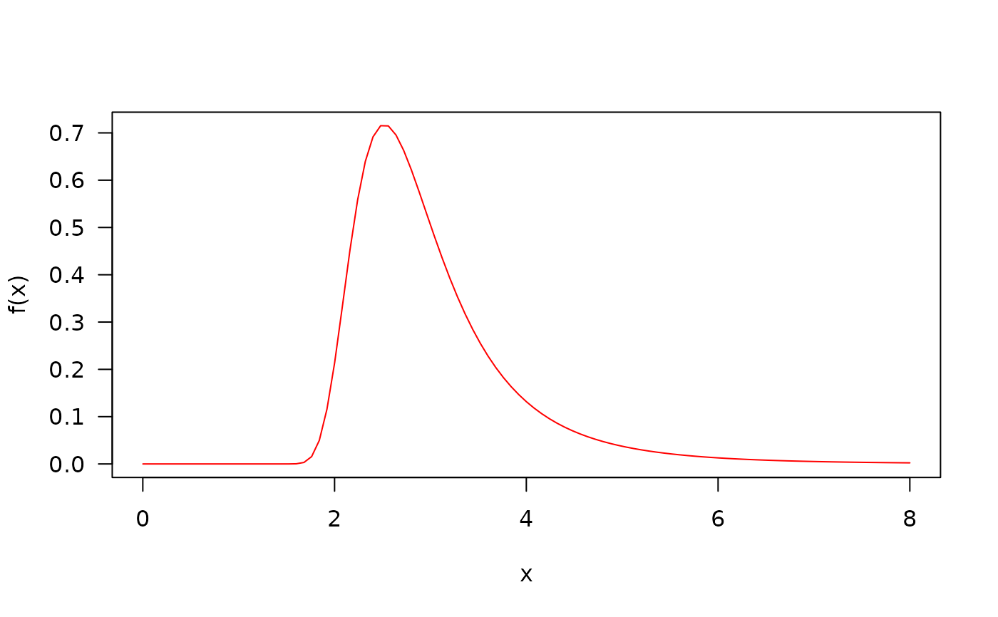
## The probability density function
curve(dGIW(x, mu=3, sigma=5, nu=0.5), from=0.001, to=8,
col="red", ylab="f(x)", las=1)
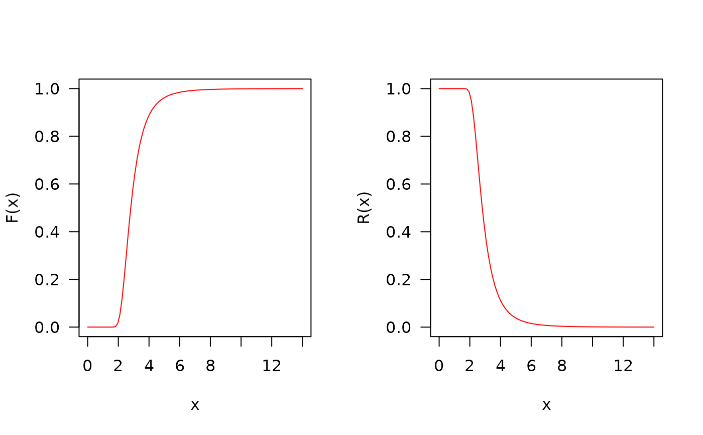
 ## The cumulative distribution and the Reliability function
par(mfrow=c(1, 2))
curve(pGIW(x, mu=3, sigma=5, nu=0.5),
from=0.0001, to=14, col="red", las=1, ylab="F(x)")
curve(pGIW(x, mu=3, sigma=5, nu=0.5, lower.tail=FALSE),
from=0.0001, to=14, col="red", las=1, ylab="R(x)")
## The cumulative distribution and the Reliability function
par(mfrow=c(1, 2))
curve(pGIW(x, mu=3, sigma=5, nu=0.5),
from=0.0001, to=14, col="red", las=1, ylab="F(x)")
curve(pGIW(x, mu=3, sigma=5, nu=0.5, lower.tail=FALSE),
from=0.0001, to=14, col="red", las=1, ylab="R(x)")
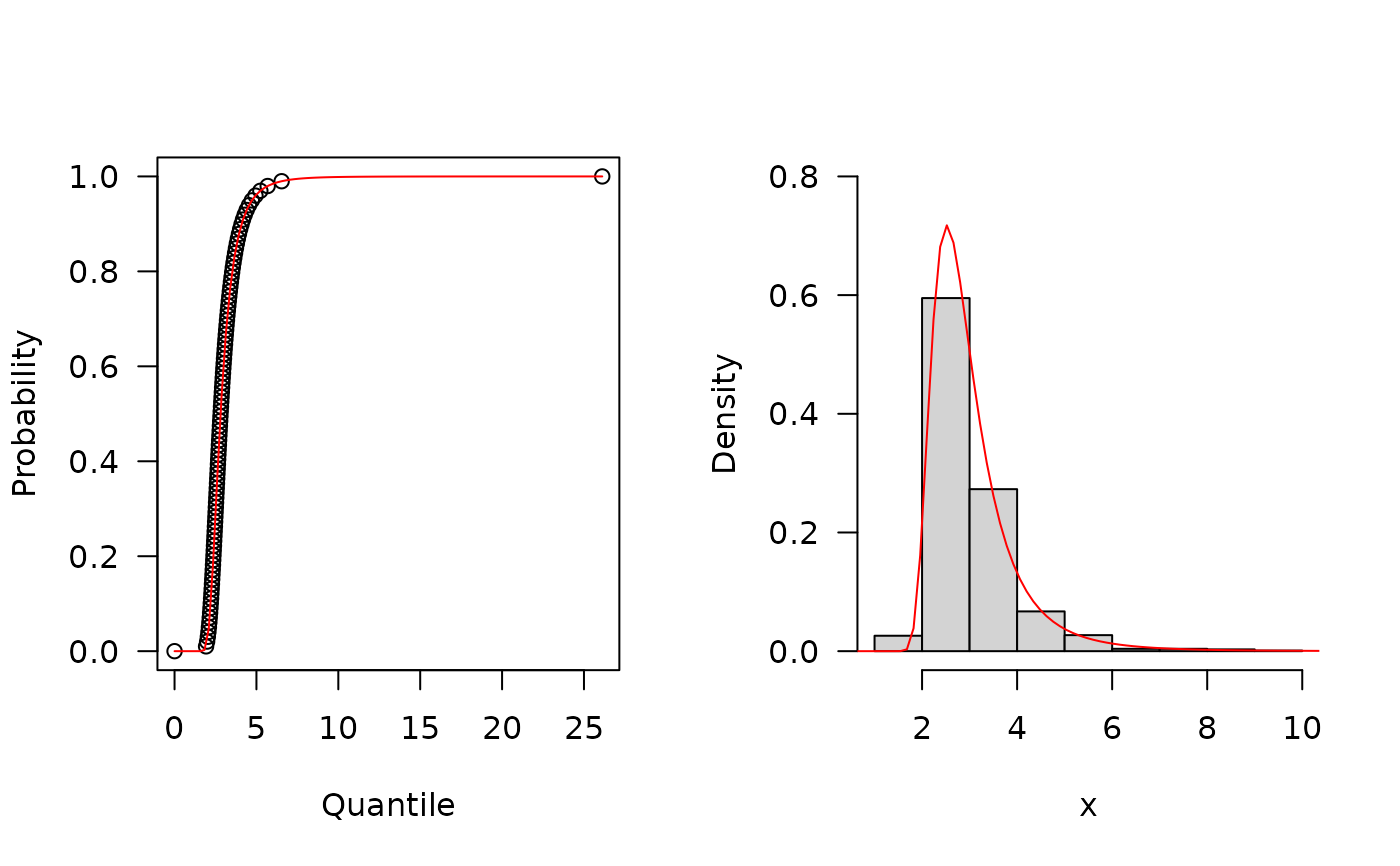
 ## The quantile function
p <- seq(from=0, to=0.99999, length.out=100)
plot(x=qGIW(p, mu=3, sigma=5, nu=0.5), y=p, xlab="Quantile",
las=1, ylab="Probability")
curve(pGIW(x, mu=3, sigma=5, nu=0.5),
from=0, add=TRUE, col="red")
## The random function
hist(rGIW(n=1000, mu=3, sigma=5, nu=0.5), freq=FALSE,
xlab="x", ylim=c(0, 0.8), las=1, main="")
curve(dGIW(x, mu=3, sigma=5, nu=0.5),
from=0.001, to=14, add=TRUE, col="red")
## The quantile function
p <- seq(from=0, to=0.99999, length.out=100)
plot(x=qGIW(p, mu=3, sigma=5, nu=0.5), y=p, xlab="Quantile",
las=1, ylab="Probability")
curve(pGIW(x, mu=3, sigma=5, nu=0.5),
from=0, add=TRUE, col="red")
## The random function
hist(rGIW(n=1000, mu=3, sigma=5, nu=0.5), freq=FALSE,
xlab="x", ylim=c(0, 0.8), las=1, main="")
curve(dGIW(x, mu=3, sigma=5, nu=0.5),
from=0.001, to=14, add=TRUE, col="red")
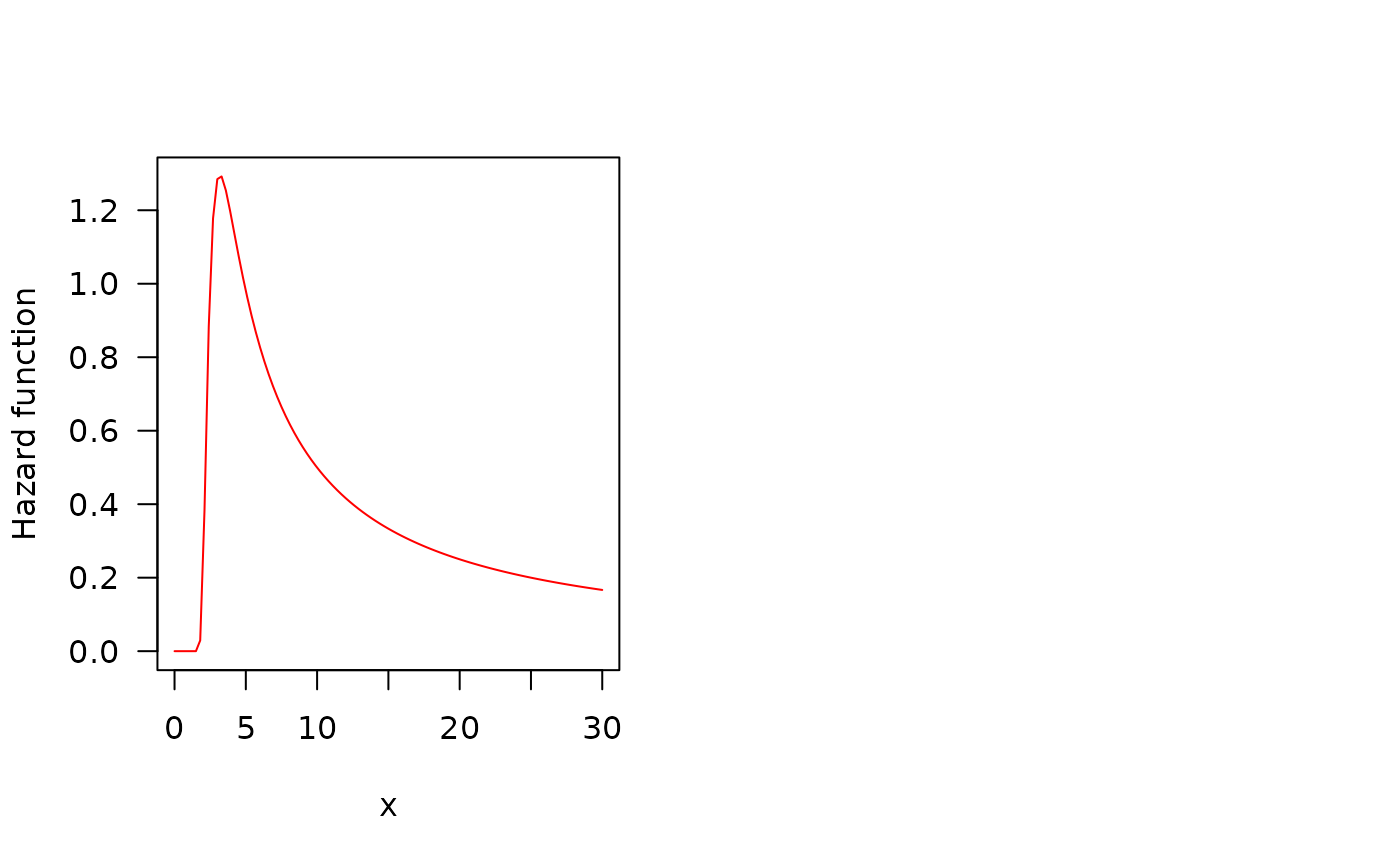
 ## The Hazard function
curve(hGIW(x, mu=3, sigma=5, nu=0.5), from=0.001, to=30,
col="red", ylab="Hazard function", las=1)
par(old_par) # restore previous graphical parameters
## The Hazard function
curve(hGIW(x, mu=3, sigma=5, nu=0.5), from=0.001, to=30,
col="red", ylab="Hazard function", las=1)
par(old_par) # restore previous graphical parameters