Density, distribution function, quantile function,
random generation and hazard function for the exponentiated XLindley distribution with
parameters mu and sigma.
Usage
dEXL(x, mu, sigma, log = FALSE)

pEXL(q, mu, sigma, log.p = FALSE, lower.tail = TRUE)

qEXL(p, mu, sigma, lower.tail = TRUE, log.p = FALSE)

rEXL(n, mu, sigma)
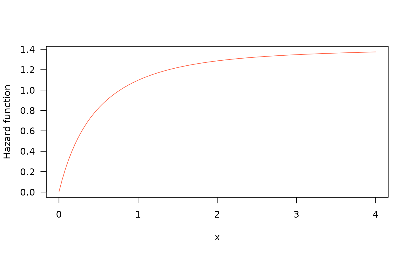
hEXL(x, mu, sigma, log = FALSE)Value
dEXL gives the density, pEXL gives the distribution
function, qEXL gives the quantile function, rEXL
generates random deviates and hEXL gives the hazard function.
Details
The exponentiated XLindley with parameters mu and sigma
has density given by
\( f(x) = \frac{\sigma\mu^2(2+\mu + x)\exp(-\mu x)}{(1+\mu)^2}\left[1- \left(1+\frac{\mu x}{(1 + \mu)^2}\right) \exp(-\mu x)\right] ^ {\sigma-1} \)
for \(x \geq 0\), \(\mu \geq 0\) and \(\sigma \geq 0\).
Note: In this implementation we changed the original parameters \(\delta\) for \(\mu\) and \(\alpha\) for \(\sigma\), we did it to implement this distribution within gamlss framework.
References
Alomair, A. M., Ahmed, M., Tariq, S., Ahsan-ul-Haq, M., & Talib, J. (2024). An exponentiated XLindley distribution with properties, inference and applications. Heliyon, 10(3).
Author
Manuel Gutierrez Tangarife, mgutierrezta@unal.edu.co
Examples
#Example 1
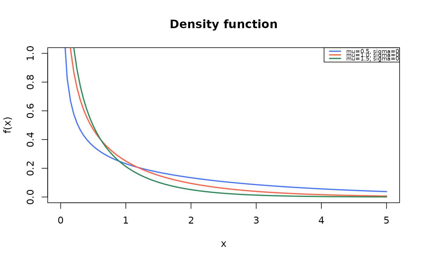
#Plotting the mass function for different parameter values
curve(dEXL(x, mu=0.5, sigma=0.5),
from=0.001, to=5,
ylim=c(0, 1),
col="royalblue1", lwd=2,
main="Density function",
xlab="x", ylab="f(x)")
curve(dEXL(x, mu=1, sigma=0.5),
col="tomato",
lwd=2,
add=TRUE)
curve(dEXL(x, mu=1.5, sigma=0.5),
col="seagreen",
lwd=2,
add=TRUE)
legend("topright", legend=c("mu=0.5, sigma=0.5",
"mu=1.0, sigma=0.5",
"mu=1.5, sigma=0.5"),
col=c("royalblue1", "tomato", "seagreen"), lwd=2, cex=0.6)
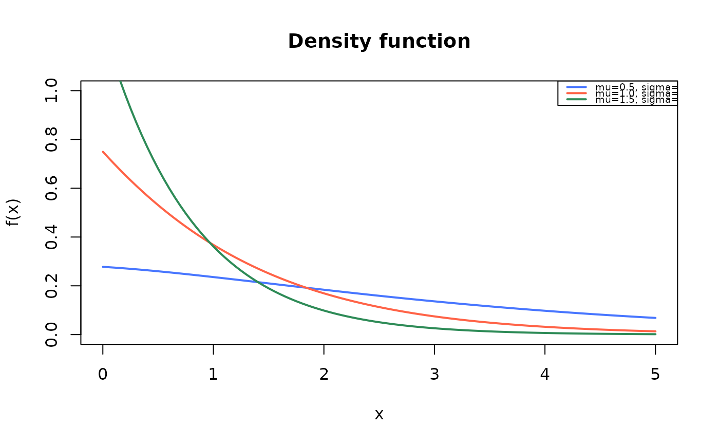
 curve(dEXL(x, mu=0.5, sigma=1),
from=0.001, to=5,
ylim=c(0, 1),
col="royalblue1", lwd=2,
main="Density function",
xlab="x", ylab="f(x)")
curve(dEXL(x, mu=1, sigma=1),
col="tomato",
lwd=2,
add=TRUE)
curve(dEXL(x, mu=1.5, sigma=1),
col="seagreen",
lwd=2,
add=TRUE)
legend("topright", legend=c("mu=0.5, sigma=1",
"mu=1.0, sigma=1",
"mu=1.5, sigma=1"),
col=c("royalblue1", "tomato", "seagreen"), lwd=2, cex=0.6)
curve(dEXL(x, mu=0.5, sigma=1),
from=0.001, to=5,
ylim=c(0, 1),
col="royalblue1", lwd=2,
main="Density function",
xlab="x", ylab="f(x)")
curve(dEXL(x, mu=1, sigma=1),
col="tomato",
lwd=2,
add=TRUE)
curve(dEXL(x, mu=1.5, sigma=1),
col="seagreen",
lwd=2,
add=TRUE)
legend("topright", legend=c("mu=0.5, sigma=1",
"mu=1.0, sigma=1",
"mu=1.5, sigma=1"),
col=c("royalblue1", "tomato", "seagreen"), lwd=2, cex=0.6)
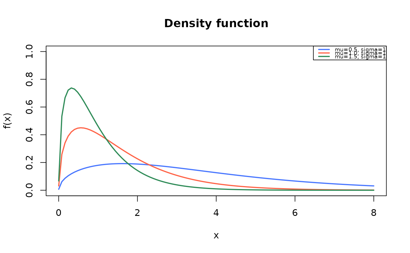
 curve(dEXL(x, mu=0.5, sigma=1.5),
from=0.001, to=8,
ylim=c(0, 1),
col="royalblue1", lwd=2,
main="Density function",
xlab="x", ylab="f(x)")
curve(dEXL(x, mu=1, sigma=1.5),
col="tomato",
lwd=2,
add=TRUE)
curve(dEXL(x, mu=1.5, sigma=1.5),
col="seagreen",
lwd=2,
add=TRUE)
legend("topright", legend=c("mu=0.5, sigma=1.5",
"mu=1.0, sigma=1.5",
"mu=1.5, sigma=1.5"),
col=c("royalblue1", "tomato", "seagreen"), lwd=2, cex=0.6)
curve(dEXL(x, mu=0.5, sigma=1.5),
from=0.001, to=8,
ylim=c(0, 1),
col="royalblue1", lwd=2,
main="Density function",
xlab="x", ylab="f(x)")
curve(dEXL(x, mu=1, sigma=1.5),
col="tomato",
lwd=2,
add=TRUE)
curve(dEXL(x, mu=1.5, sigma=1.5),
col="seagreen",
lwd=2,
add=TRUE)
legend("topright", legend=c("mu=0.5, sigma=1.5",
"mu=1.0, sigma=1.5",
"mu=1.5, sigma=1.5"),
col=c("royalblue1", "tomato", "seagreen"), lwd=2, cex=0.6)
 # Example 2
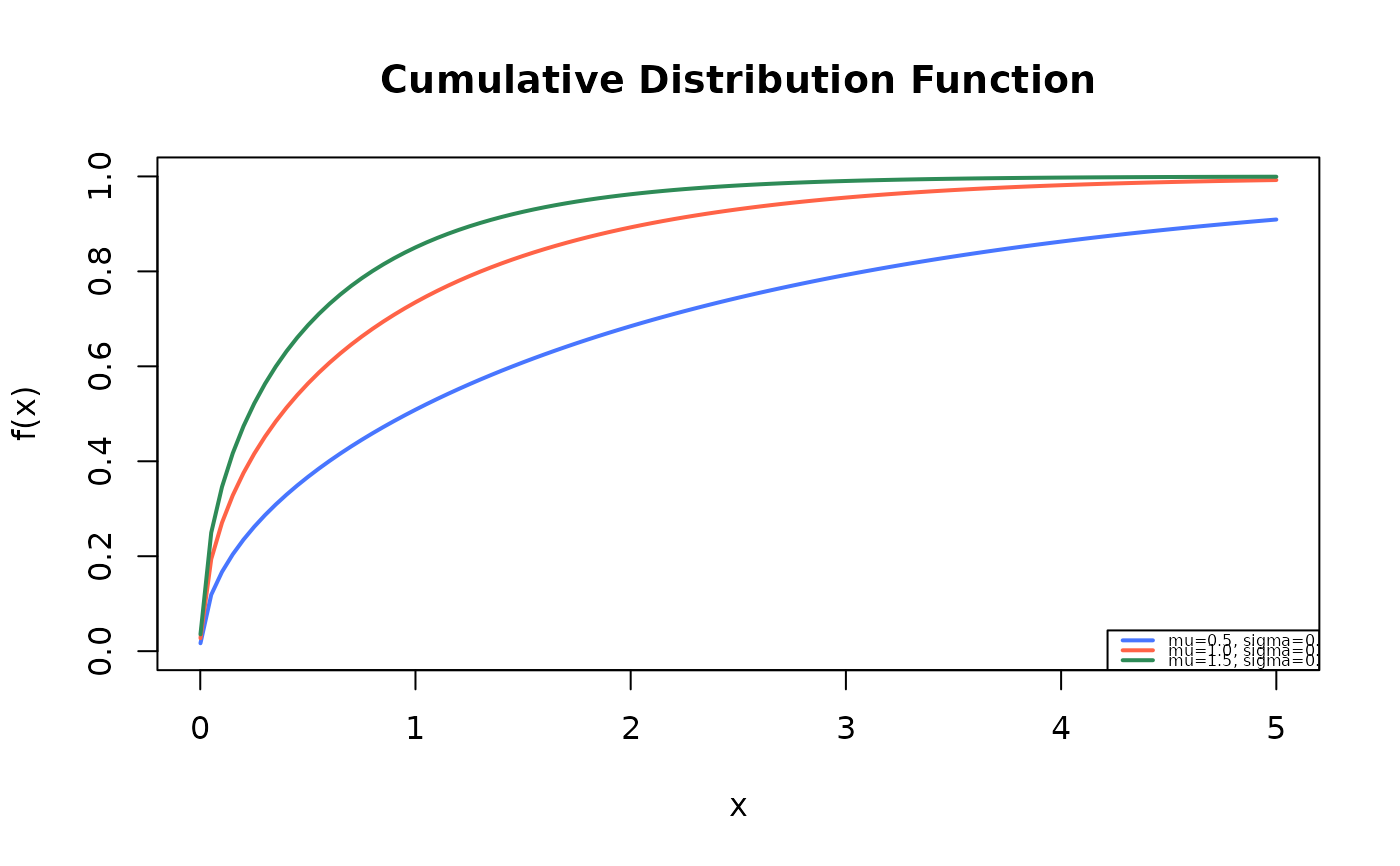
# Checking if the cumulative curves converge to 1
curve(pEXL(x, mu=0.5, sigma=0.5),
from=0.001, to=5,
ylim=c(0, 1),
col="royalblue1", lwd=2,
main="Cumulative Distribution Function",
xlab="x", ylab="f(x)")
curve(pEXL(x, mu=1, sigma=0.5),
col="tomato",
lwd=2,
add=TRUE)
curve(pEXL(x, mu=1.5, sigma=0.5),
col="seagreen",
lwd=2,
add=TRUE)
legend("bottomright", legend=c("mu=0.5, sigma=0.5",
"mu=1.0, sigma=0.5",
"mu=1.5, sigma=0.5"),
col=c("royalblue1", "tomato", "seagreen"), lwd=2, cex=0.5)
# Example 2
# Checking if the cumulative curves converge to 1
curve(pEXL(x, mu=0.5, sigma=0.5),
from=0.001, to=5,
ylim=c(0, 1),
col="royalblue1", lwd=2,
main="Cumulative Distribution Function",
xlab="x", ylab="f(x)")
curve(pEXL(x, mu=1, sigma=0.5),
col="tomato",
lwd=2,
add=TRUE)
curve(pEXL(x, mu=1.5, sigma=0.5),
col="seagreen",
lwd=2,
add=TRUE)
legend("bottomright", legend=c("mu=0.5, sigma=0.5",
"mu=1.0, sigma=0.5",
"mu=1.5, sigma=0.5"),
col=c("royalblue1", "tomato", "seagreen"), lwd=2, cex=0.5)
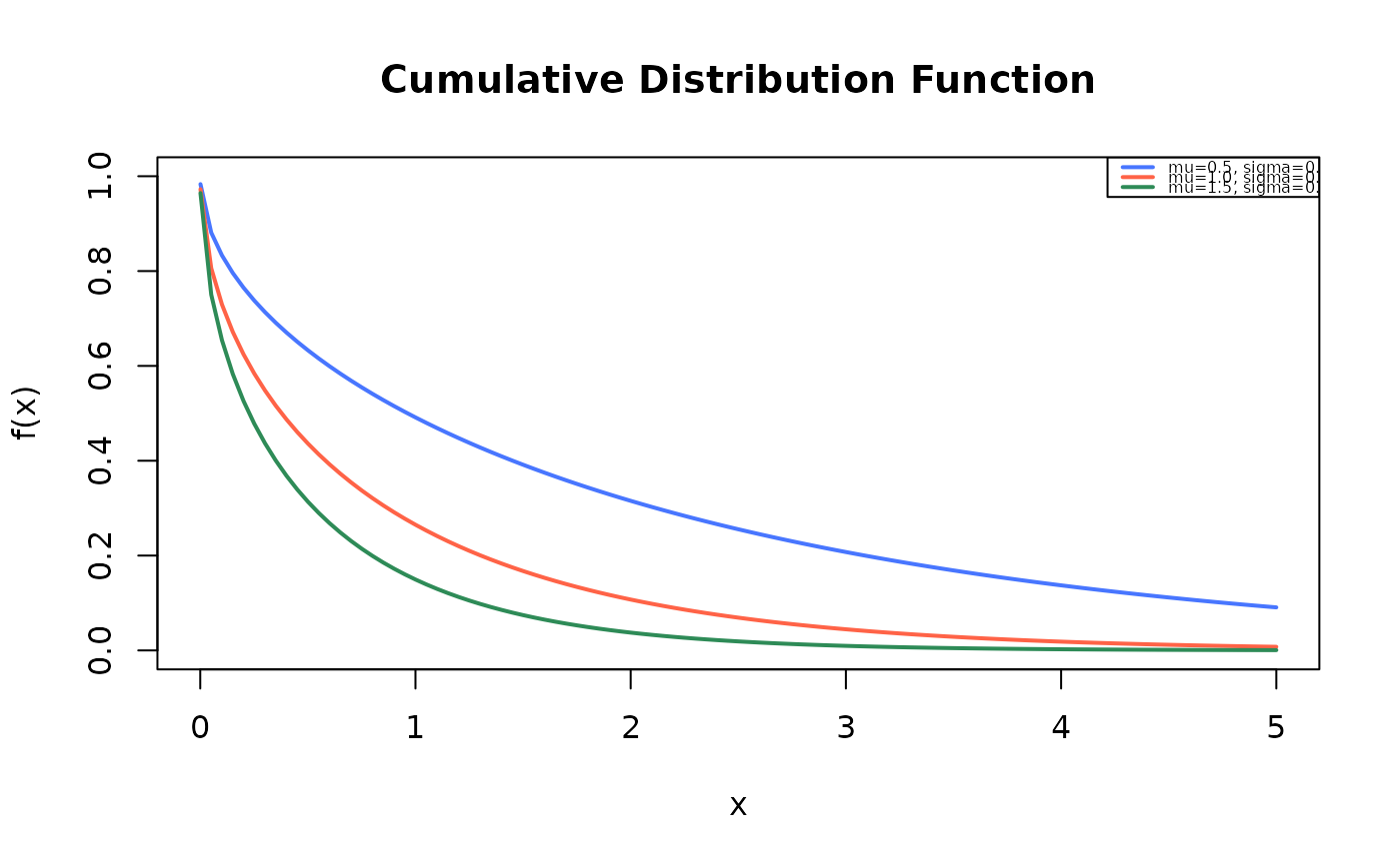
 curve(pEXL(x, mu=0.5, sigma=0.5, lower.tail=FALSE),
from=0.001, to=5,
ylim=c(0, 1),
col="royalblue1", lwd=2,
main="Cumulative Distribution Function",
xlab="x", ylab="f(x)")
curve(pEXL(x, mu=1, sigma=0.5, lower.tail=FALSE),
col="tomato",
lwd=2,
add=TRUE)
curve(pEXL(x, mu=1.5, sigma=0.5, lower.tail=FALSE),
col="seagreen",
lwd=2,
add=TRUE)
legend("topright", legend=c("mu=0.5, sigma=0.5",
"mu=1.0, sigma=0.5",
"mu=1.5, sigma=0.5"),
col=c("royalblue1", "tomato", "seagreen"), lwd=2, cex=0.5)
curve(pEXL(x, mu=0.5, sigma=0.5, lower.tail=FALSE),
from=0.001, to=5,
ylim=c(0, 1),
col="royalblue1", lwd=2,
main="Cumulative Distribution Function",
xlab="x", ylab="f(x)")
curve(pEXL(x, mu=1, sigma=0.5, lower.tail=FALSE),
col="tomato",
lwd=2,
add=TRUE)
curve(pEXL(x, mu=1.5, sigma=0.5, lower.tail=FALSE),
col="seagreen",
lwd=2,
add=TRUE)
legend("topright", legend=c("mu=0.5, sigma=0.5",
"mu=1.0, sigma=0.5",
"mu=1.5, sigma=0.5"),
col=c("royalblue1", "tomato", "seagreen"), lwd=2, cex=0.5)
 #example 3
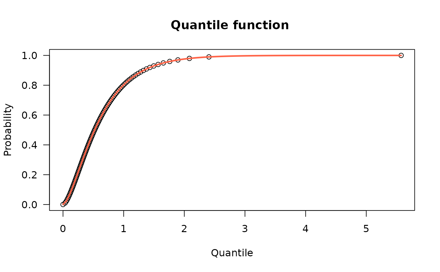
## The quantile function
p <- seq(from=0, to=0.99999, length.out=100)
plot(x=qEXL(p, mu=2.3, sigma=1.7), y=p, xlab="Quantile",
las=1, ylab="Probability", main="Quantile function ")
curve(pEXL(x, mu=2.3, sigma=1.7),
from=0, add=TRUE, col="tomato", lwd=2.5)
#example 3
## The quantile function
p <- seq(from=0, to=0.99999, length.out=100)
plot(x=qEXL(p, mu=2.3, sigma=1.7), y=p, xlab="Quantile",
las=1, ylab="Probability", main="Quantile function ")
curve(pEXL(x, mu=2.3, sigma=1.7),
from=0, add=TRUE, col="tomato", lwd=2.5)
 #some values
p <- c(0.25, 0.5, 0.75)
quantile <- qEXL(p=p, mu=2.3, sigma=1.7)
for(i in quantile){
print(integrate(dEXL, lower=0, upper=i, mu=2.3, sigma=1.7))
}
#> 0.2500001 with absolute error < 4.9e-05
#> 0.5 with absolute error < 4.4e-05
#> 0.7500001 with absolute error < 0.00012
#example 4
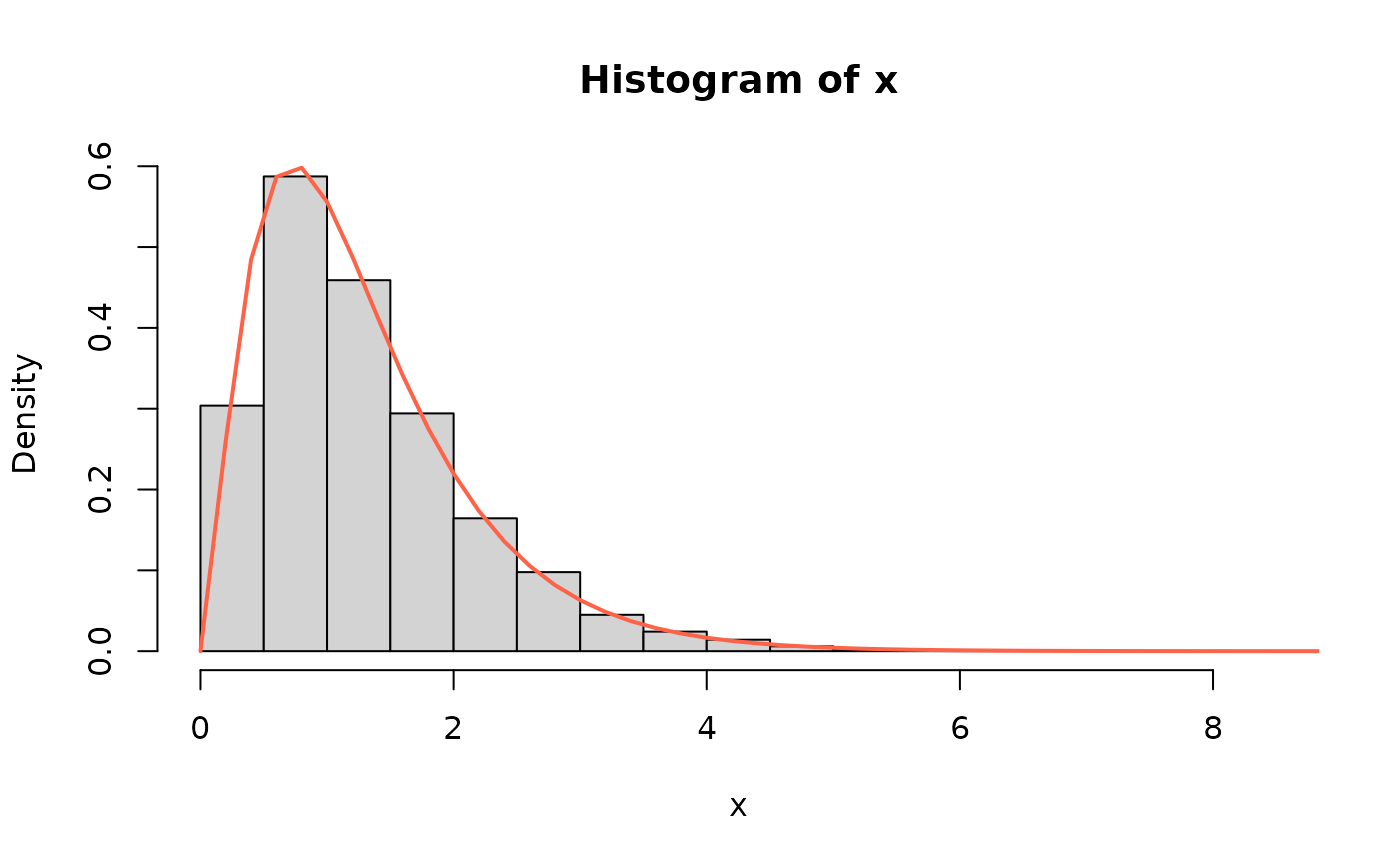
## The random function
x <- rEXL(n=10000, mu=1.5, sigma=2.5)
hist(x, freq=FALSE)
curve(dEXL(x, mu=1.5, sigma=2.5), from=0, to=20,
add=TRUE, col="tomato", lwd=2)
#some values
p <- c(0.25, 0.5, 0.75)
quantile <- qEXL(p=p, mu=2.3, sigma=1.7)
for(i in quantile){
print(integrate(dEXL, lower=0, upper=i, mu=2.3, sigma=1.7))
}
#> 0.2500001 with absolute error < 4.9e-05
#> 0.5 with absolute error < 4.4e-05
#> 0.7500001 with absolute error < 0.00012
#example 4
## The random function
x <- rEXL(n=10000, mu=1.5, sigma=2.5)
hist(x, freq=FALSE)
curve(dEXL(x, mu=1.5, sigma=2.5), from=0, to=20,
add=TRUE, col="tomato", lwd=2)
 #example 5
## The Hazard function
curve(hEXL(x, mu=1.5, sigma=2), from=0.001, to=4,
col="tomato", ylab="Hazard function", las=1)
#example 5
## The Hazard function
curve(hEXL(x, mu=1.5, sigma=2), from=0.001, to=4,
col="tomato", ylab="Hazard function", las=1)