Density, distribution function, quantile function,
random generation and hazard function for the Extended Odd Fr?chet-Nadarajah-Haghighi distribution
with parameters mu, sigma, nu and tau.
Usage
dEOFNH(x, mu, sigma, nu, tau, log = FALSE)

pEOFNH(q, mu, sigma, nu, tau, lower.tail = TRUE, log.p = FALSE)

qEOFNH(p, mu, sigma, nu, tau, lower.tail = TRUE, log.p = FALSE)

rEOFNH(n, mu, sigma, nu, tau)

hEOFNH(x, mu, sigma, nu, tau)Value
dEOFNH gives the density, pEOFNH gives the distribution
function, qEOFNH gives the quantile function, rEOFNH
generates random numbers and hEOFNH gives the hazard function.
Details
Tthe Extended Odd Frechet-Nadarajah-Haghighi mu,
sigma, nu and tau has density given by
\(f(x)= \frac{\mu\sigma\nu\tau(1+\nu x)^{\sigma-1}e^{(1-(1+\nu x)^\sigma)}[1-(1-e^{(1-(1+\nu x)^\sigma)})^{\mu}]^{\tau-1}}{(1-e^{(1-(1+\nu x)^{\sigma})})^{\mu\tau+1}} e^{-[(1-e^{(1-(1+\nu x)^\sigma)})^{-\mu}-1]^{\tau}},\)
for \(x > 0\), \(\mu > 0\), \(\sigma > 0\), \(\nu > 0\) and \(\tau > 0\).
Examples
old_par <- par(mfrow = c(1, 1)) # save previous graphical parameters
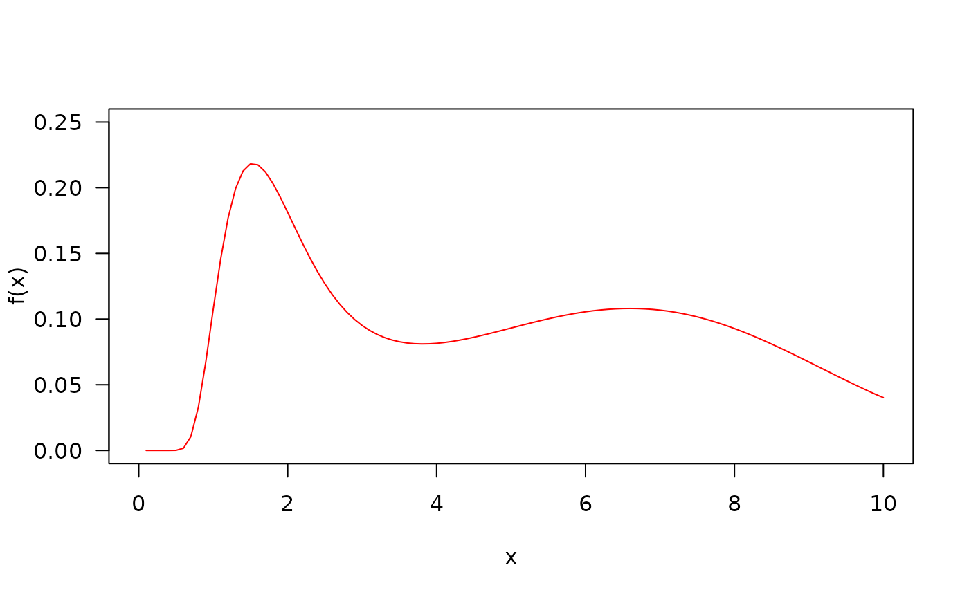
##The probability density function
par(mfrow=c(1,1))
curve(dEOFNH(x, mu=18.5, sigma=5.1, nu=0.1, tau=0.1), from=0, to=10,
ylim=c(0, 0.25), col="red", las=1, ylab="f(x)")
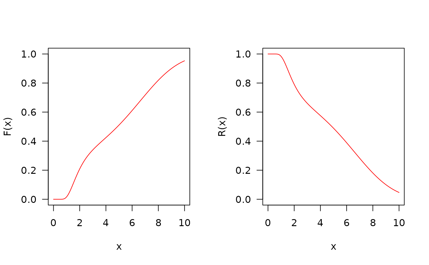
 ## The cumulative distribution and the Reliability function
par(mfrow = c(1, 2))
curve(pEOFNH(x,mu=18.5, sigma=5.1, nu=0.1, tau=0.1), from = 0, to = 10,
ylim = c(0, 1), col = "red", las = 1, ylab = "F(x)")
curve(pEOFNH(x, mu=18.5, sigma=5.1, nu=0.1, tau=0.1, lower.tail = FALSE),
from = 0, to = 10, ylim = c(0, 1), col = "red", las = 1, ylab = "R(x)")
## The cumulative distribution and the Reliability function
par(mfrow = c(1, 2))
curve(pEOFNH(x,mu=18.5, sigma=5.1, nu=0.1, tau=0.1), from = 0, to = 10,
ylim = c(0, 1), col = "red", las = 1, ylab = "F(x)")
curve(pEOFNH(x, mu=18.5, sigma=5.1, nu=0.1, tau=0.1, lower.tail = FALSE),
from = 0, to = 10, ylim = c(0, 1), col = "red", las = 1, ylab = "R(x)")
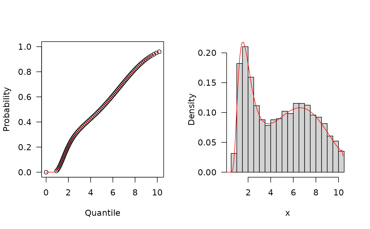
 ##The quantile function
p <- seq(from=0, to=0.99999, length.out=100)
plot(x=qEOFNH(p, mu=18.5, sigma=5.1, nu=0.1, tau=0.1), y=p, xlab="Quantile",
las=1, ylab="Probability")
curve(pEOFNH(x, mu=18.5, sigma=5.1, nu=0.1, tau=0.1), from=0, add=TRUE, col="red")
##The random function
hist(rEOFNH(n=10000, mu=18.5, sigma=5.1, nu=0.1, tau=0.1), freq=FALSE,
xlab="x", las=1, main="")
curve(dEOFNH(x, mu=18.5, sigma=5.1, nu=0.1, tau=0.1), from=0, add=TRUE, col="red", ylim=c(0,1.25))
##The quantile function
p <- seq(from=0, to=0.99999, length.out=100)
plot(x=qEOFNH(p, mu=18.5, sigma=5.1, nu=0.1, tau=0.1), y=p, xlab="Quantile",
las=1, ylab="Probability")
curve(pEOFNH(x, mu=18.5, sigma=5.1, nu=0.1, tau=0.1), from=0, add=TRUE, col="red")
##The random function
hist(rEOFNH(n=10000, mu=18.5, sigma=5.1, nu=0.1, tau=0.1), freq=FALSE,
xlab="x", las=1, main="")
curve(dEOFNH(x, mu=18.5, sigma=5.1, nu=0.1, tau=0.1), from=0, add=TRUE, col="red", ylim=c(0,1.25))
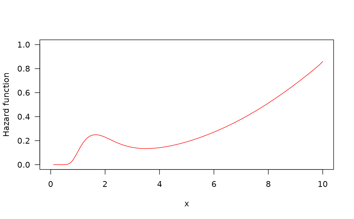
 ##The Hazard function
par(mfrow=c(1,1))
curve(hEOFNH(x, mu=18.5, sigma=5.1, nu=0.1, tau=0.1), from=0, to=10, ylim=c(0, 1),
col="red", ylab="Hazard function", las=1)
##The Hazard function
par(mfrow=c(1,1))
curve(hEOFNH(x, mu=18.5, sigma=5.1, nu=0.1, tau=0.1), from=0, to=10, ylim=c(0, 1),
col="red", ylab="Hazard function", las=1)
 par(old_par) # restore previous graphical parameters