Density, distribution function, quantile function,
random generation and hazard function for the Exponentiated Modifien Weibull Extension distribution
with parameters mu, sigma, nu and tau.
Usage
dEMWEx(x, mu, sigma, nu, tau, log = FALSE)

pEMWEx(q, mu, sigma, nu, tau, lower.tail = TRUE, log.p = FALSE)

qEMWEx(p, mu, sigma, nu, tau, lower.tail = TRUE, log.p = FALSE)

rEMWEx(n, mu, sigma, nu, tau)

hEMWEx(x, mu, sigma, nu, tau)Value
dEMWEx gives the density, pEMWEx gives the distribution
function, qEMWEx gives the quantile function, rEMWEx
generates random deviates and hEMWEx gives the hazard function.
Details
The Exponentiated Modifien Weibull Extension Distribution with parameters mu,
sigma, nu and tau has density given by
\(f(x)= \nu \sigma \tau (\frac{x}{\mu})^{\sigma-1} \exp((\frac{x}{\mu})^\sigma + \nu \mu (1- \exp((\frac{x}{\mu})^\sigma))) (1 - \exp (\nu\mu (1- \exp((\frac{x}{\mu})^\sigma))))^{\tau-1} ,\)
for \(x > 0\), \(\nu> 0\), \(\mu > 0\), \(\sigma> 0\) and \(\tau > 0\).
Author
Johan David Marin Benjumea, johand.marin@udea.edu.co
Examples
old_par <- par(mfrow = c(1, 1)) # save previous graphical parameters
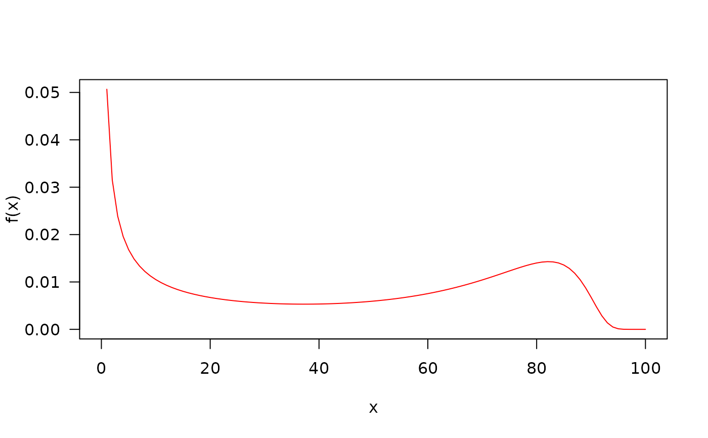
## The probability density function
curve(dEMWEx(x, mu = 49.046, sigma =3.148, nu=0.00005, tau=0.1), from=0, to=100,
col = "red", las = 1, ylab = "f(x)")
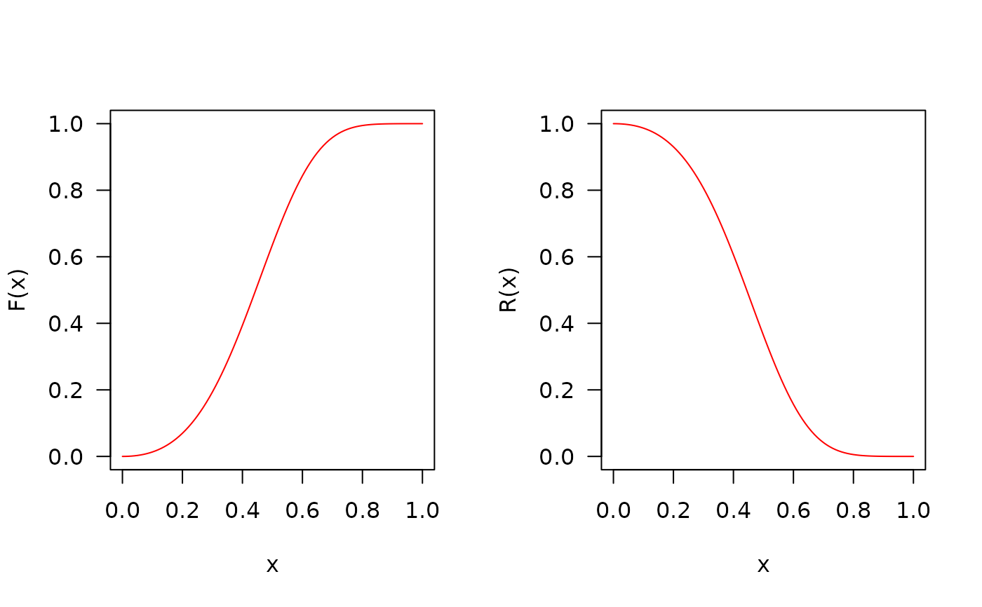
 ## The cumulative distribution and the Reliability function
par(mfrow = c(1, 2))
curve(pEMWEx(x, mu = (1/4), sigma =1, nu=1, tau=2), from = 0, to = 1,
ylim = c(0, 1), col = "red", las = 1, ylab = "F(x)")
curve(pEMWEx(x, mu = (1/4), sigma =1, nu=1, tau=2, lower.tail = FALSE),
from = 0, to = 1, ylim = c(0, 1), col = "red", las = 1, ylab = "R(x)")
## The cumulative distribution and the Reliability function
par(mfrow = c(1, 2))
curve(pEMWEx(x, mu = (1/4), sigma =1, nu=1, tau=2), from = 0, to = 1,
ylim = c(0, 1), col = "red", las = 1, ylab = "F(x)")
curve(pEMWEx(x, mu = (1/4), sigma =1, nu=1, tau=2, lower.tail = FALSE),
from = 0, to = 1, ylim = c(0, 1), col = "red", las = 1, ylab = "R(x)")
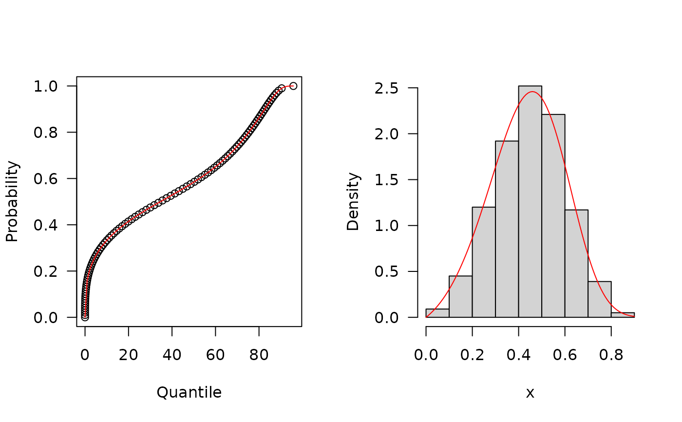
 ## The quantile function
p <- seq(from = 0, to = 0.99999, length.out = 100)
plot(x = qEMWEx(p = p, mu = 49.046, sigma =3.148, nu=0.00005, tau=0.1), y = p,
xlab = "Quantile", las = 1, ylab = "Probability")
curve(pEMWEx(x, mu = 49.046, sigma =3.148, nu=0.00005, tau=0.1), from = 0, add = TRUE,
col = "red")
## The random function
hist(rEMWEx(1000, mu = (1/4), sigma =1, nu=1, tau=2), freq = FALSE, xlab = "x",
las = 1, main = "")
curve(dEMWEx(x, mu = (1/4), sigma =1, nu=1, tau=2), from = 0, add = TRUE,
col = "red", ylim = c(0, 0.5))
## The quantile function
p <- seq(from = 0, to = 0.99999, length.out = 100)
plot(x = qEMWEx(p = p, mu = 49.046, sigma =3.148, nu=0.00005, tau=0.1), y = p,
xlab = "Quantile", las = 1, ylab = "Probability")
curve(pEMWEx(x, mu = 49.046, sigma =3.148, nu=0.00005, tau=0.1), from = 0, add = TRUE,
col = "red")
## The random function
hist(rEMWEx(1000, mu = (1/4), sigma =1, nu=1, tau=2), freq = FALSE, xlab = "x",
las = 1, main = "")
curve(dEMWEx(x, mu = (1/4), sigma =1, nu=1, tau=2), from = 0, add = TRUE,
col = "red", ylim = c(0, 0.5))
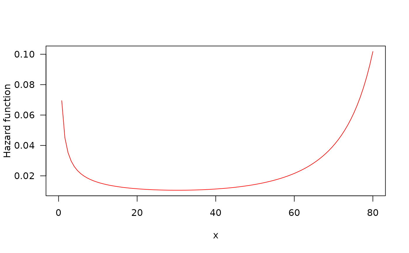
 ## The Hazard function(
par(mfrow=c(1,1))
curve(hEMWEx(x, mu = 49.046, sigma =3.148, nu=0.00005, tau=0.1), from = 0, to = 80,
col = "red", ylab = "Hazard function", las = 1)
## The Hazard function(
par(mfrow=c(1,1))
curve(hEMWEx(x, mu = 49.046, sigma =3.148, nu=0.00005, tau=0.1), from = 0, to = 80,
col = "red", ylab = "Hazard function", las = 1)
 par(old_par) # restore previous graphical parameters