Density, distribution function, quantile function,
random generation and hazard function for the Additive Weibull distribution
with parameters mu, sigma, nu and tau.
Usage
dAddW(x, mu, sigma, nu, tau, log = FALSE)

pAddW(q, mu, sigma, nu, tau, lower.tail = TRUE, log.p = FALSE)

qAddW(p, mu, sigma, nu, tau, lower.tail = TRUE, log.p = FALSE)

rAddW(n, mu, sigma, nu, tau)

hAddW(x, mu, sigma, nu, tau)
Arguments
- x, q
vector of quantiles.
- mu
parameter.
- sigma
parameter.
- nu
shape parameter.
- tau
shape parameter.
- log, log.p
logical; if TRUE, probabilities p are given as log(p).
- lower.tail
logical; if TRUE (default), probabilities are P[X <= x], otherwise, P[X > x].
- p
vector of probabilities.
- n
number of observations.
Value
dAddW gives the density, pAddW gives the distribution
function, qAddW gives the quantile function, rAddW
generates random deviates and hAddW gives the hazard function.
Details
Additive Weibull Distribution with parameters mu,
sigma, nu and tau has density given by
\(f(x) = (\mu\nu x^{\nu - 1} + \sigma\tau x^{\tau - 1}) \exp({-\mu x^{\nu} - \sigma x^{\tau} }),\)
for x > 0.
Author
Amylkar Urrea Montoya, amylkar.urrea@udea.edu.co
Examples
old_par <- par(mfrow = c(1, 1)) # save previous graphical parameters
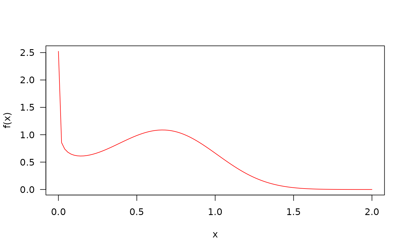
## The probability density function
curve(dAddW(x, mu=1.5, sigma=0.5, nu=3, tau=0.8), from=0.0001, to=2,
col="red", las=1, ylab="f(x)")
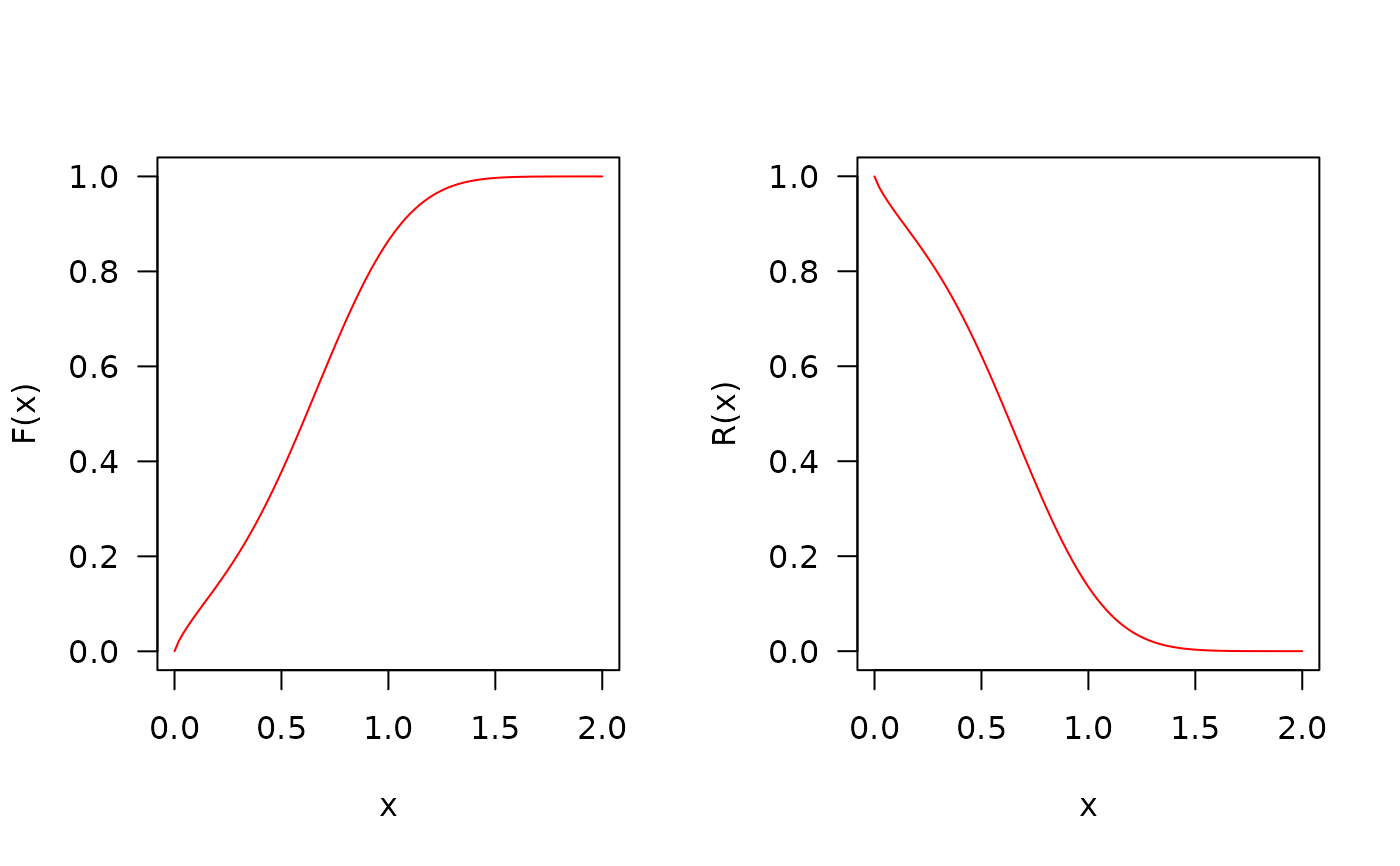
 ## The cumulative distribution and the Reliability function
par(mfrow=c(1, 2))
curve(pAddW(x, mu=1.5, sigma=0.5, nu=3, tau=0.8),
from=0.0001, to=2, col="red", las=1, ylab="F(x)")
curve(pAddW(x, mu=1.5, sigma=0.5, nu=3, tau=0.8, lower.tail=FALSE),
from=0.0001, to=2, col="red", las=1, ylab="R(x)")
## The cumulative distribution and the Reliability function
par(mfrow=c(1, 2))
curve(pAddW(x, mu=1.5, sigma=0.5, nu=3, tau=0.8),
from=0.0001, to=2, col="red", las=1, ylab="F(x)")
curve(pAddW(x, mu=1.5, sigma=0.5, nu=3, tau=0.8, lower.tail=FALSE),
from=0.0001, to=2, col="red", las=1, ylab="R(x)")
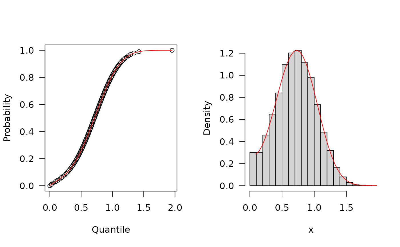
 ## The quantile function
p <- seq(from=0, to=0.99999, length.out=100)
plot(x=qAddW(p, mu=1.5, sigma=0.2, nu=3, tau=0.8), y=p, xlab="Quantile",
las=1, ylab="Probability")
curve(pAddW(x, mu=1.5, sigma=0.2, nu=3, tau=0.8),
from=0, add=TRUE, col="red")
## The random function
hist(rAddW(n=10000, mu=1.5, sigma=0.2, nu=3, tau=0.8), freq=FALSE,
xlab="x", las=1, main="")
curve(dAddW(x, mu=1.5, sigma=0.2, nu=3, tau=0.8),
from=0.09, to=5, add=TRUE, col="red")
## The quantile function
p <- seq(from=0, to=0.99999, length.out=100)
plot(x=qAddW(p, mu=1.5, sigma=0.2, nu=3, tau=0.8), y=p, xlab="Quantile",
las=1, ylab="Probability")
curve(pAddW(x, mu=1.5, sigma=0.2, nu=3, tau=0.8),
from=0, add=TRUE, col="red")
## The random function
hist(rAddW(n=10000, mu=1.5, sigma=0.2, nu=3, tau=0.8), freq=FALSE,
xlab="x", las=1, main="")
curve(dAddW(x, mu=1.5, sigma=0.2, nu=3, tau=0.8),
from=0.09, to=5, add=TRUE, col="red")
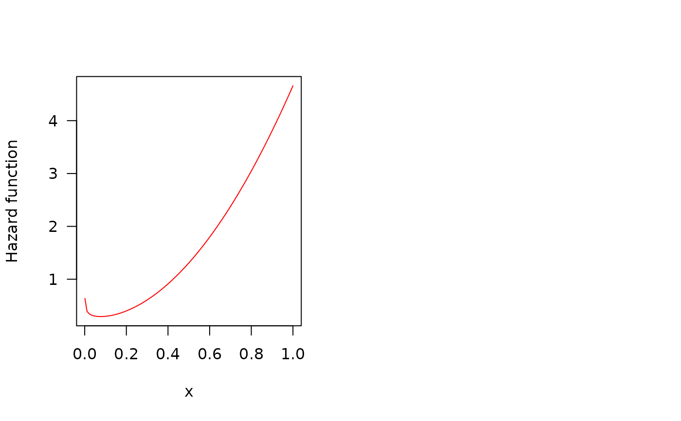
 ## The Hazard function
curve(hAddW(x, mu=1.5, sigma=0.2, nu=3, tau=0.8), from=0.001, to=1,
col="red", ylab="Hazard function", las=1)
par(old_par) # restore previous graphical parameters
## The Hazard function
curve(hAddW(x, mu=1.5, sigma=0.2, nu=3, tau=0.8), from=0.001, to=1,
col="red", ylab="Hazard function", las=1)
par(old_par) # restore previous graphical parameters